How to reverse names in Excel

You can watch a video tutorial here.

Excel is frequently used as a database and can store data in any format that you choose. There may be a case where you have a list of names in which the first name is followed by the last name. You may need to reverse this order to sort the names according to surname. 

There are 2 ways of doing this, one way is a static method which has to be repeated each time the names need to be reversed. The second is a dynamic method using a formula that automatically reverses the name even if the name changes.

1. Use the Flash Fill option as the static method
2. Build a dynamic formula using the MID(), SEARCH() and LEN() functions:
   • MID() function: this returns a specified number of characters from a string
     1. Syntax: MID(text, start number, number of characters)
        1. text: the string from which the characters are to be extracted
        2. start number: the number of the character from which the extraction is to start
        3. number of characters: the number of characters to extract
   • SEARCH() function: this returns the position of the character being searched for within a string
     1. Syntax: SEARCH(character, text, start)
        1. Character: the character to be located
        2. text: the string in which the character is to be found
        3. start number (optional): the position from which the search is to start 
   • LEN() function: this returns the length or the number of characters in a string
     1. Syntax: LEN(text)
     2. text: the string for which the length is to be computed

Option 1 – Use Flash Fill

Step 1 – Create the pattern

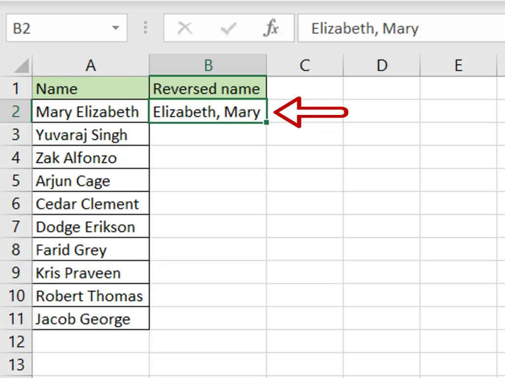
• Select the cell where the result is to be displayed
• Type the following:
  • Elizabeth, Mary
• Press Enter

Step 2 – Use Flash Fill

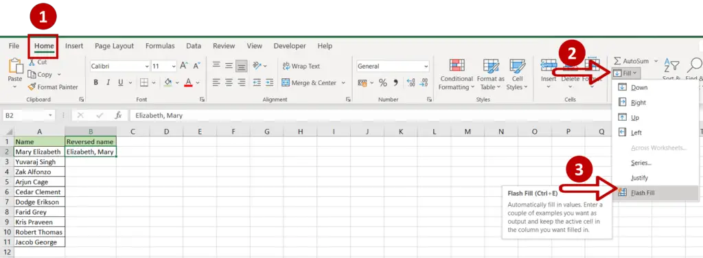
• Go to Home > Editing
• Expand the Fill drop-down
• Select Flash Fill

Step 3 – Check the result

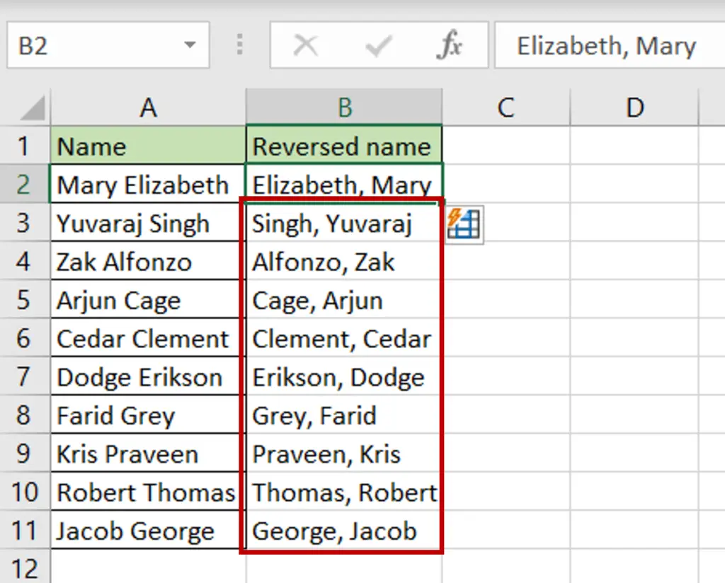
• The same pattern is applied to the rest of the names
• The names are reversed

Option 2 – Build a formula

Step 1 – Create the formula

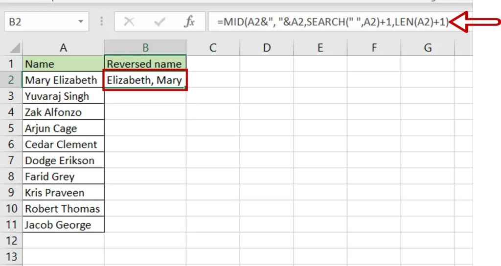
• Select the cell in which the result is to appear
• Type the formula using cell references:

=MID(Name &”, “&Name,SEARCH(” “,Name)+1,LEN(Name)+1)

• The first argument duplicates the name and adds a comma:
  • Name &”, “&Name  = Mary Elizabeth, Mary Elizabeth
• The second argument searches for the first space in the name and adds 1 to return the starting position of the string to be extracted:
  • SEARCH(” “, Name)+1 = 6
• The third argument specifies the number of characters to be extracted which is the length of the text plus 1 for the comma:
  • LEN(Name)+1 = 15
• Press Enter

Step 2 – Copy the formula

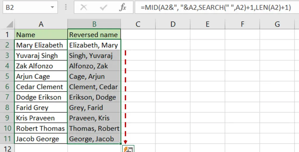
• Select the cell with the formula
• Using the fill handle from the first cell, drag the formula to the remaining cells

OR

1. Select the cell with the formula and press Ctrl+C or choose Copy from the context menu (right-click)
2. Select the rest of the cells in the column and press Ctrl+V or choose Paste from the context menu (right-click)

Step 3 – Check the result

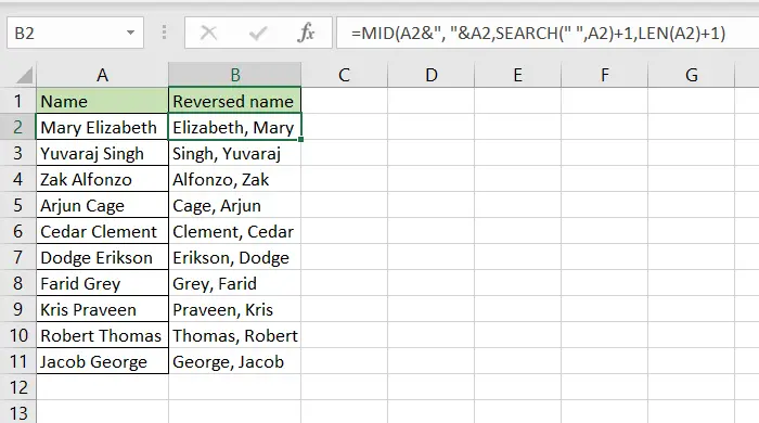
• The formula is copied to the rest of the cells
• The names are reversed