
How to reverse a column in Excel
 By
SpreadCheaters
By
SpreadCheaters
You can watch a video tutorial here.
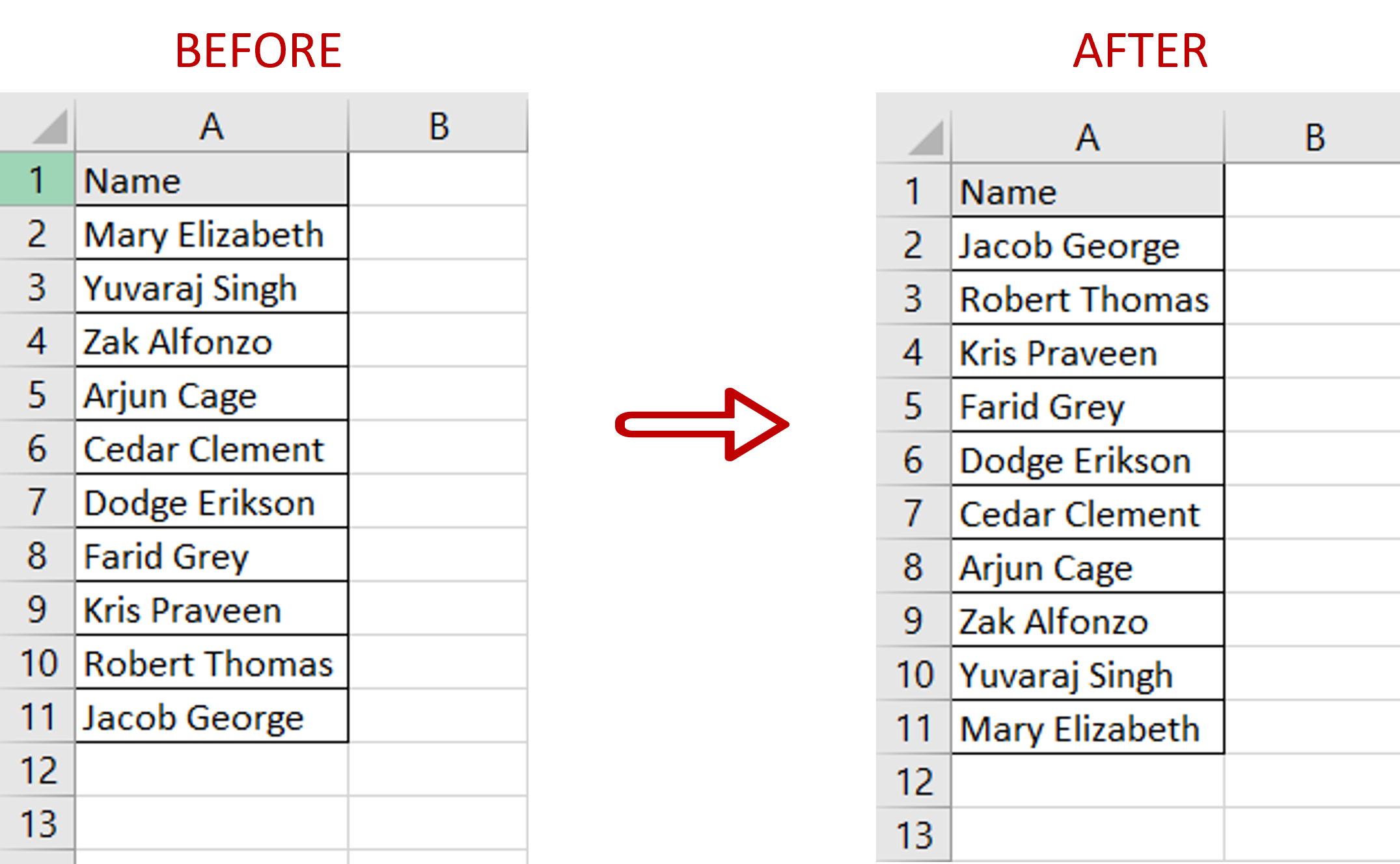
Excel provides a simple way to sort a table based on any one of its columns. Text data can be sorted in ascending or descending alphabetical order and numbers can also be sorted in ascending or descending order. What happens in situations where there is no defined order to a column and it needs to be reversed? In such situations, there is a workaround.
Step 1 – Create a blank column
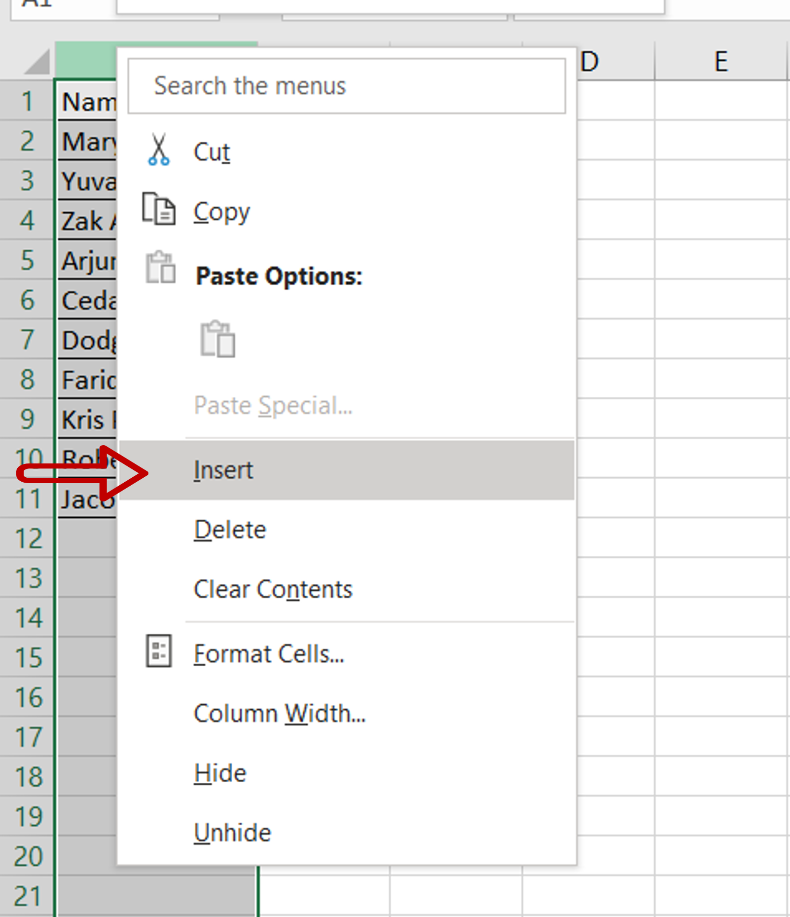
– Select the first column
– Right-click and select Insert from the context menu
Step 2 – Create a pattern for serial numbers
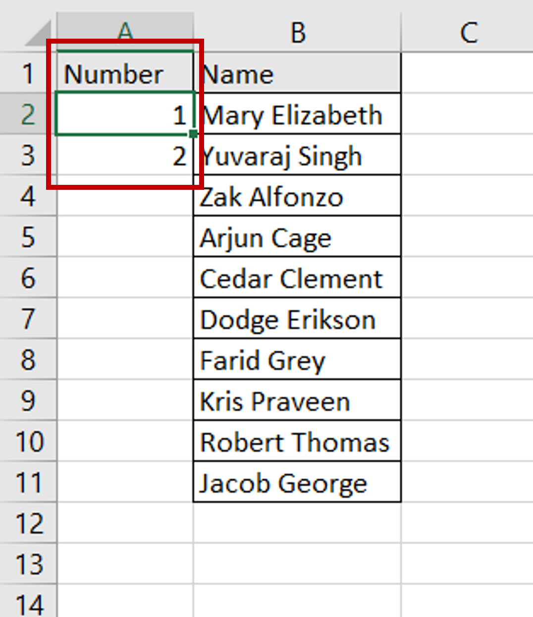
– Name the new column ‘Number’
– Type ‘1’ in the first cell of the ‘Number’ column
– Type 2 in the second cell of the ‘Number’ column
Step 3 – Copy the list to the rest of the column
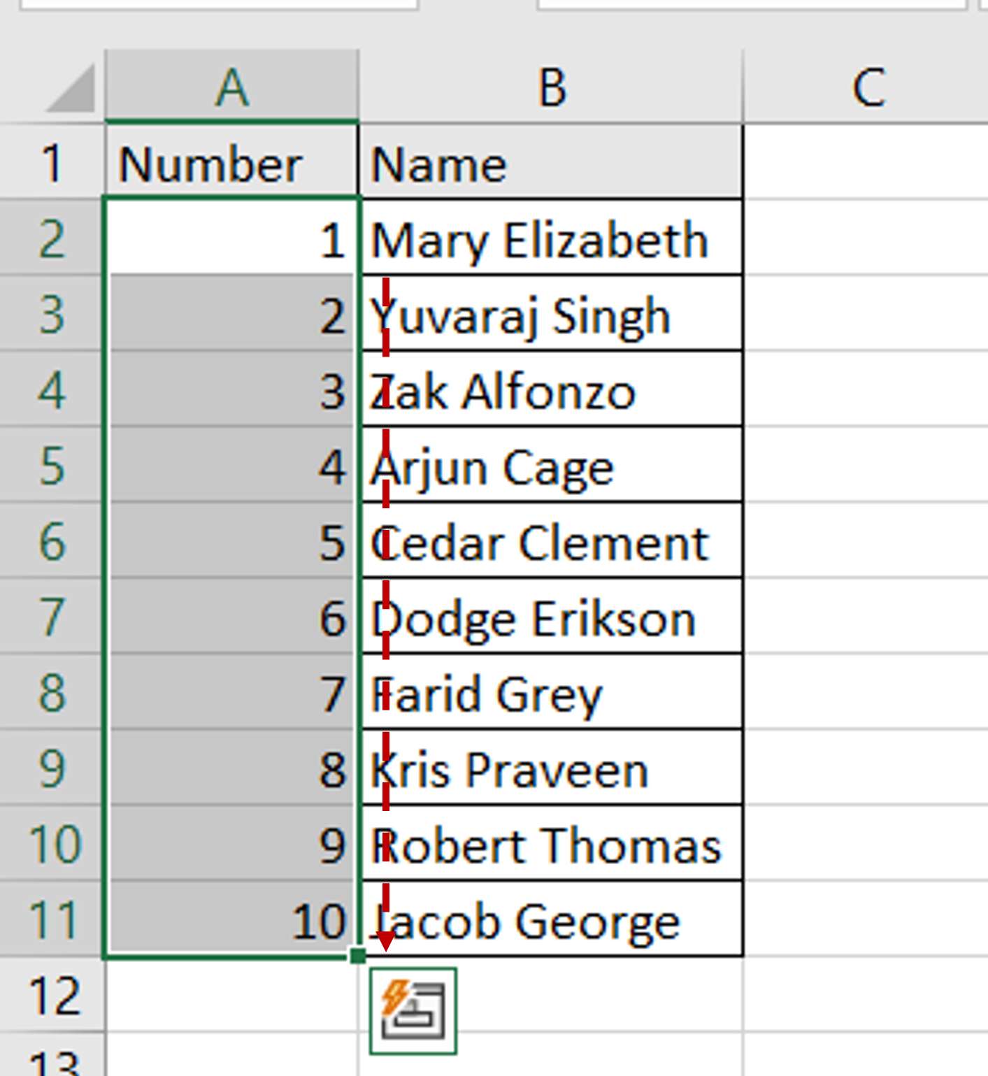
– Select the first two cells in the ‘Number’ column
– Using the fill handle from the second cell, drag the formula to the remaining cells
OR
a) Select the cell with the formula and press Ctrl+C or choose Copy from the context menu (right-click)
b) Select the rest of the cells in the column and press Ctrl+V or choose Paste from the context menu (right-click)
Step 4 – Open the sort box
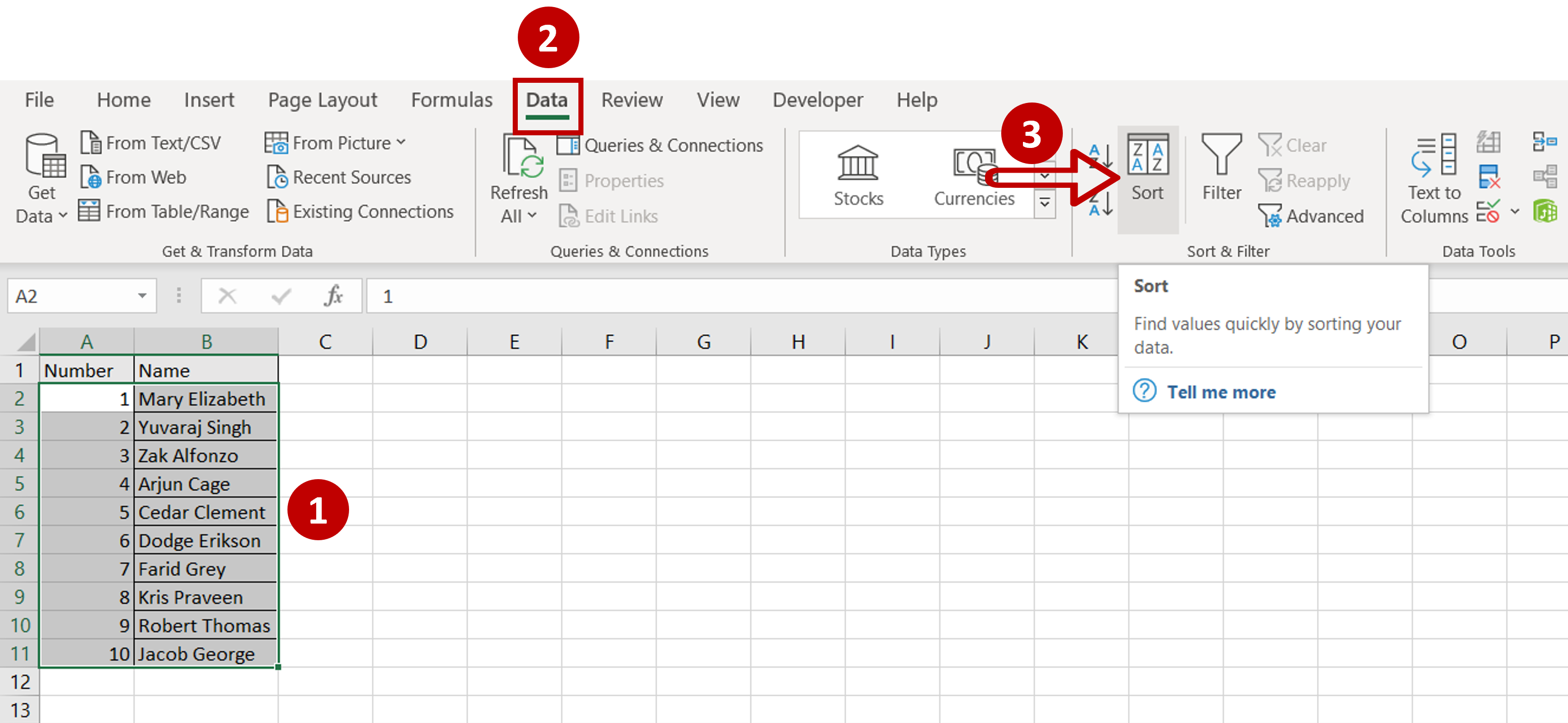
– Select the data
– Choose the Sort option from the ribbon under Home > Sort & Filter
Step 5 – Set the parameters
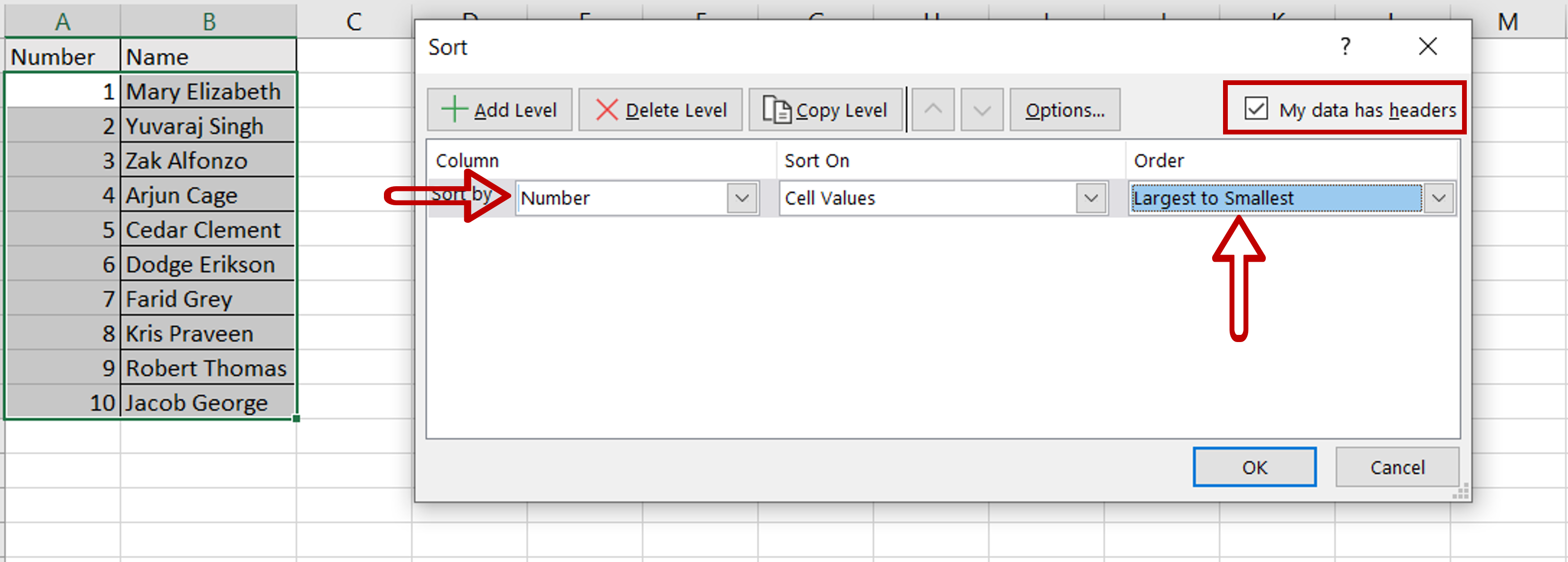
– Define the parameters:
>Sort: ‘Number’
>Order: Largest to Smallest
>My data has headers: Tick
– Click OK
Step 6 – Delete the extra column
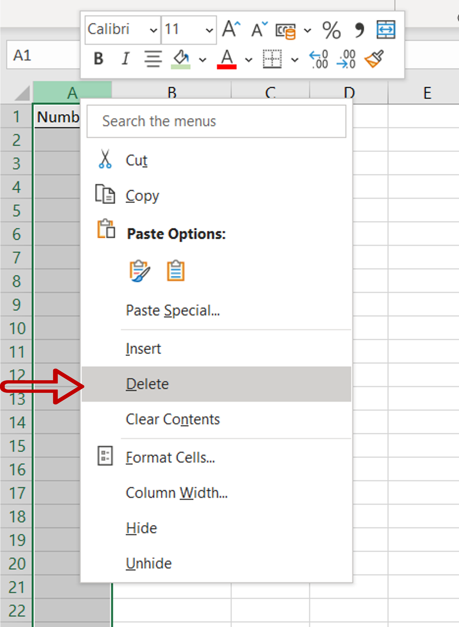
– Select the ‘Number’ column
– Right-click and select Delete from the context menu
– Click OK
Step 7 – Check the result

– The column is reversed and the rows are displayed in reverse order


