How to remove vertical lines in Excel

In Excel, vertical lines typically refer to the vertical gridlines that appear in a worksheet to separate columns. These gridlines are used to visually separate columns and make it easier to read data in a table. Vertical lines in Excel can improve your spreadsheets’ readability, aesthetics, organization, and usability. Using the gridlines makes it easier to ensure that data is entered into the correct cell

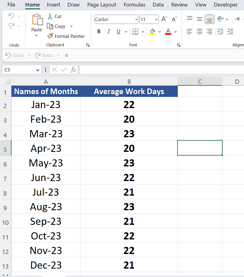
In this tutorial, we will learn how to remove vertical lines in Excel. The following data shows the month’s names in a year and the total work days in those months. Consider the following data set to learn how to remove vertical lines in Excel.

Method 1 – Removing vertical lines through the home tab

There are 2 methods to remove vertical lines in Excel. In this method, we are going to remove the vertical lines in Excel through the home tab. Follow the given steps to learn how to remove vertical lines.

Step 1 – Select the columns

• Select the columns in which you want the vertical lines to be hidden.
• If you want to remove vertical lines from the whole worksheet, press CTRL + A, but we are going to only hide some specific columns but the method will be the same.

Step 2 – Go to the home tab

• Click on the Home tab.
• Click on the format option, in the cells group.

Step 3 – Select the Format cells option

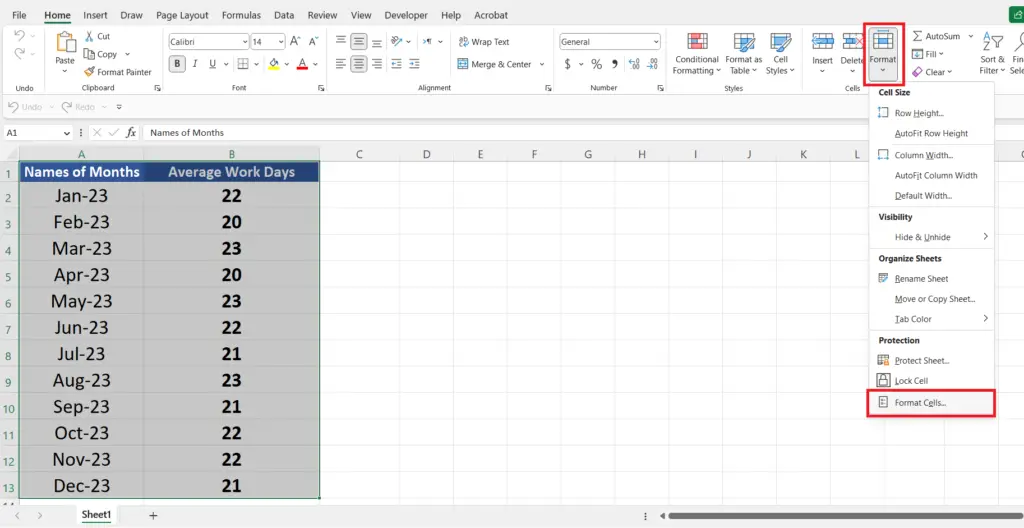
• When you click on the Format option in the cells group, a drop-down menu will appear.
• From that drop-down menu select the format cells option.

Step 4 – Click on the borders

• When you click on the format cells option, a format cells dialogue box will appear.
• Click on the borders tab.

Step 5 – Choose an appropriate option.

• Choose an appropriate option from the dialogue box
• Or you can simply click on the diagram to remove gridlines.
• Click OK to confirm that you want to remove the lines.

Method 2 – Removing vertical lines from the context menu

In this method, we are going to remove the vertical lines by using the context menu. This method is similar to the method above but the difference is that we are going to use a context menu.

Step 1 – Select the columns or worksheet

• Select the columns in which you want the vertical lines to be hidden, we are selecting the whole worksheet, by pressing CTRL + A.
• After selecting the worksheet, right-click.

Step 2 – Click on format cells

• From that context menu, choose format cell
• This will display the same format cells dialogue box.

Step 3 – Choose an appropriate option.

• From that dialogue box select any option.
• Click OK to confirm that you have removed the vertical gridlines.