How to remove the VLOOKUP formula in Microsoft Excel

Removing the VLOOKUP function in Excel refers to the process of eliminating the formula while preserving the resulting values. This means that the function will no longer be active and cannot alter the retrieved results. [1] 

In this tutorial, we will learn how to remove the VLOOKUP function[2]  in Microsoft Excel. One of the commonly used methods to remove the VLOOKUP function in Microsoft Excel is through the Paste Special feature. Additionally, there are alternative methods available such as keyboard shortcut keys or utilizing the right-click function with the cursor.

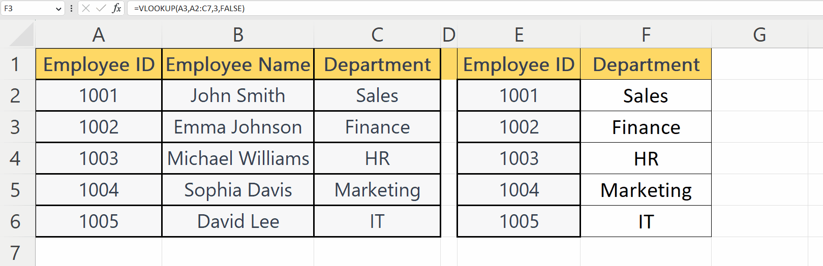
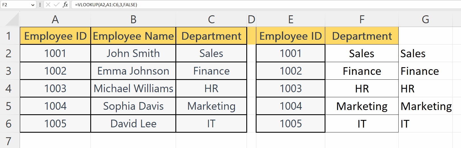
Right now we have employed the VLOOKUP function to extract the department of some employees utilizing the employee IDs. We aim to remove the VLOOKUP function.[3] 

Method 1: Utilizing the Paste Special Feature

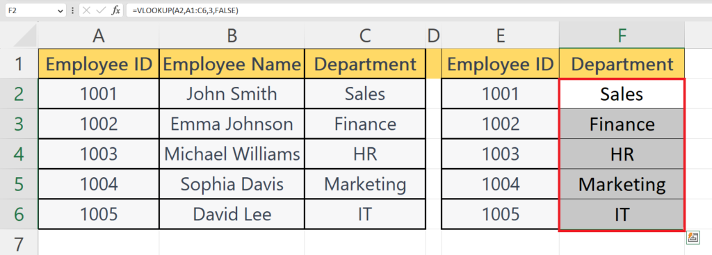
Step 1 – Copy the Cells with VLOOKUP

• Copy the cells containing the VLOOKUP function.
• For this, select the cell, do a right-click and choose the copy option from the context menu.

Step 2 – Perform a Right-Click on the Destination

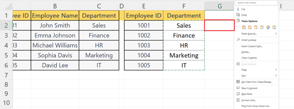
• Perform a right-click on the cell where you aim to paste the values i.e. the cells with VLOOKUP removed.

Step 3 – Choose the Paste Special Button

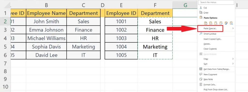
• Choose the Paste Special button.

Step 4 – Choose the Values Option and Hit the OK Button

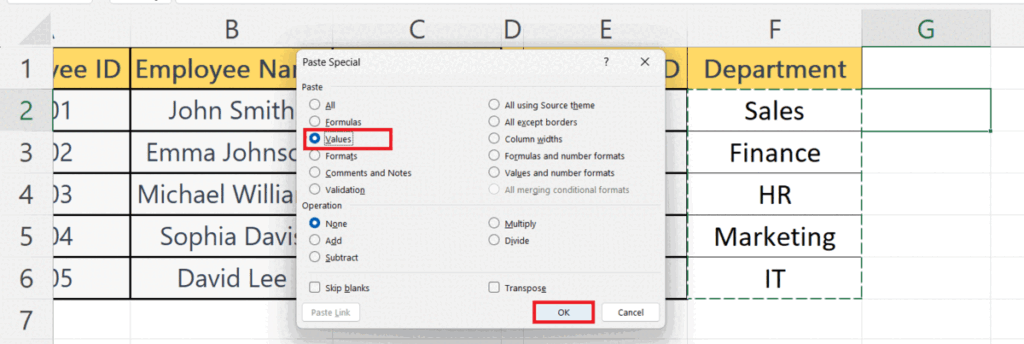
• Choose the Values option from the Paste Special dialog box.
• Hit the OK button.

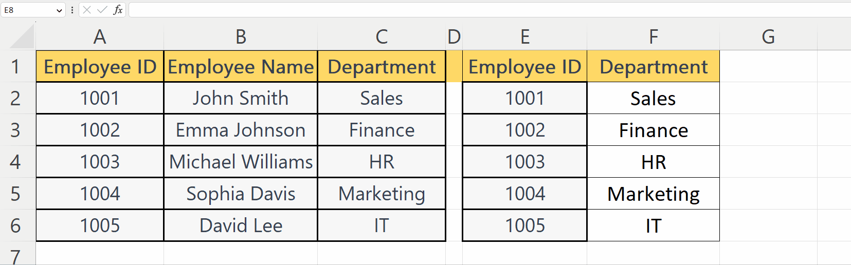
Step 5 – Now Delete the Orginal Cells

• Now delete the cells containing the VLOOKUP function.
• This can be done by selecting the cells, doing a right-click, and choosing the Delete option in the context menu.
• A small dialog box will appear after choosing the Delete option, select the “Shift cell left” option.
  

Method 2: Utilizing the Right-Click Function with the Cursor

Step 1 – Select the Cells

• Select the cells with the VLOOKUP function.

Step 2 – Press and Hold the Right-Mouse Button and Drag and Drop

• Hover the cursor over the boundary of the selection.
• Press and hold the right mouse button.
• Drag and drop to another location.

Step 3 – Choose the Option Labeled “Copy Here as Values Only”

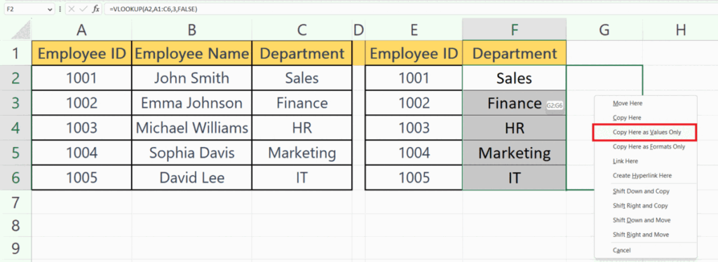
• Choose the option labeled “ Copy Here as Values Only” from the menu that appears.

Step 4 – Now Delete the Orginal Cells

• Now delete the cells containing the VLOOKUP function.
• This can be done by selecting the cells, doing a right-click, and choosing the Delete option in the context menu.
• A small dialog box will appear after choosing the Delete option, select the “Shift cell left” option.