How to remove the last digit in Excel

You can watch a video tutorial here.

Excel has several functions and tools that can be used to manipulate text and numbers.  Some of these functions can be used to modify the contents of a cell. When you are cleaning data, you may need to remove the last digit from a number as it may be just an indicator and not part of the actual number. This happens particularly when you are working with data imported from other applications. 

Here we will see how to remove the last digit in 2 ways – one by using a tool and the other by using functions. 

1. Using Flash fill
2. Using the LEFT() and LEN() functions:
   • LEFT() function: this returns a specified number of characters from the left of a string
     • Syntax: LEFT(text, number of characters)
       • text: the string from which the characters are to be extracted
       • number of characters: the number of characters to extract
   • LEN() function: this returns the length or the number of characters in a string
     • Syntax: LEN(text)
       • text: the string for which the length is to be computed

Option 1 – Use Flash Fill

Step 1 – Create the sample

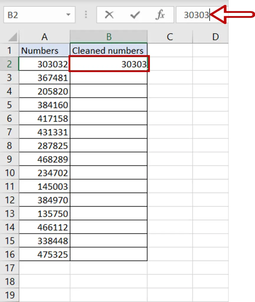
• Copy the first number using Ctrl+C
• Select the destination cell and paste the number using Ctrl+C
• Edit the cell by pressing F2 and deleting the last digit
• Press Enter

Step 2 – Choose the flash fill option

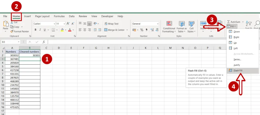
• Go to Home > Editing
• Expand the Fill menu
• Click on Flash Fill

Step 3 – Remove the flash fill options box

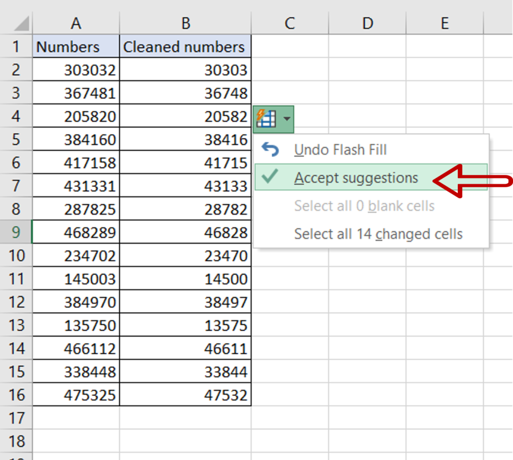
• Expand the flash fill options box
• Click Accept suggestions

Step 4 – Check the result

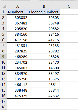
• The rest of the column is populated with the same pattern i.e. the last digit removed

Option 2 – Use the LEFT() and LEN() functions

Step 1 – Create the formula

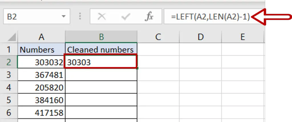
• Select the destination cell
• Type the formula using cell references:

=LEFT(Number, LEN(Number)-1)

• Press Enter

Step 2 – Copy the formula

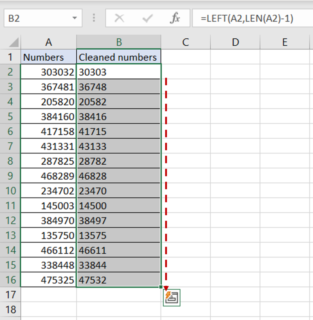
• Using the fill handle from the first cell, drag the formula to the remaining cells

OR

1. Select the cell with the formula and press Ctrl+C or choose Copy from the context menu (right-click)
2. Select the rest of the cells in the column and press Ctrl+V or choose Paste from the context menu (right-click)

Step 3 – Check the result

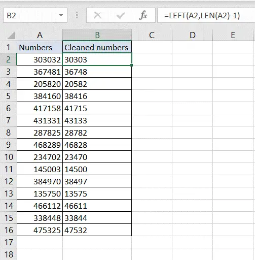
• All digits from the left are returned except for the last one