
How to remove special characters in Excel
 By
SpreadCheaters
By
SpreadCheaters
You can watch a video tutorial here.

A big challenge that many face when cleaning data imported from other applications is the removal of special characters. When cleaning up data or performing data analysis, you may need to remove all the special characters from a cell or cells. Removing each type of special character using the find & replace tool can be time-consuming and may not be wholly accurate especially when there is a large amount of data.
In this example, we will first build a lookup table that contains all the special characters to be removed. We will then build a formula using Excel functions to remove all the special characters listed in the lookup table. The approach to building the formula is explained below.
1. Create an array of numbers equal to the length of the text in the cell using the SEQUENCE() function
a. SEQUENCE(): this generates a matrix of numbers according
i. Syntax: SEQUENCE(rows, columns, start, step)
1. rows: the number of rows in the matrix
2. columns: the number of columns in the matrix
3. start: (optional)the start number
4. step: (optional) the number by which each number should increment
2. Put each character in the text into the array using the MID() function
a. MID(): this returns a specified number of characters from a string
i. Syntax: MID(text, start number, number of characters)
1. text: the string from which the characters are to be extracted
2. start number: the number of the character from which the extraction is to start
3. number of characters: the number of characters to extract
3. Find the special characters using the MATCH() and remove them using the IF() function
a. MATCH(): this searches for an item in a range and returns the position of the item in the range
i. Syntax: MATCH(value, range, type)
1. value: the item to look for
2. range: the range of cells in which to search
3. type: (optional) the type of match i.e. exact or approximate
b. IF(): this evaluates a condition and returns a value depending on whether the condition is true or false
i. Syntax: IF(condition, true, false)
1. condition: the condition or statement to be evaluated
2. true: the value to be returned if the condition is true
3. false: the value to be returned if the condition is false
4. Replace the errors with actual values using the IFERROR() function
a. IFERROR(): if a formula results in an error, this function replaces the error with a specified value
i. Syntax: IFERROR(formula,value)
1. formula: the formula to be evaluated
2. value: the value to be returned if the formula returns an error
5. Collapse the array into a single string using the TEXTJOIN() function
a. TEXTJOIN() function: this combines multiple pieces of text into a single string using the specified delimiter
i. Syntax: TEXTJOIN(delimiter, ignore_empty, text1, text 2…….)
1. delimiter: the delimiter to be used between the pieces of text
2. ignore_empty: if set to TRUE, this ignores empty pieces of text
3. text1, text 2…..: the pieces of text to be joined. At least one piece is mandatory
Note: In some versions of Excel, this formula is to be treated as an array formula. After creating the entire formula, press Ctrl+Shift+Enter instead of just Enter.
Step 1 – Create the lookup table
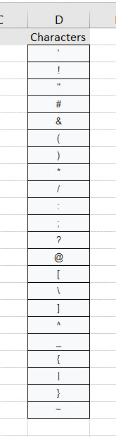
– In a column on the sheet, list all the characters to be removed
– There should be only one character in each row
Step 2 – Create an array of numbers
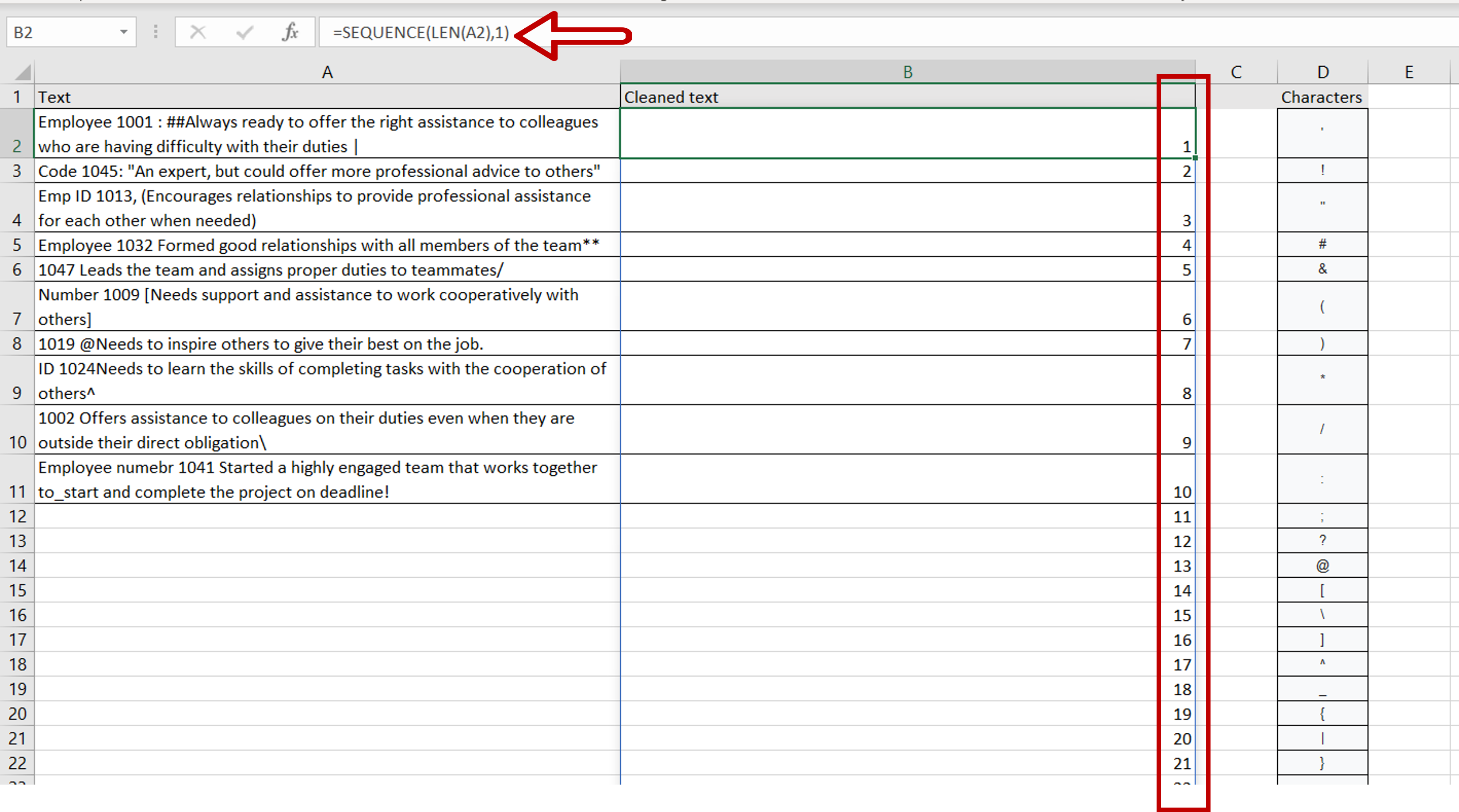
– Select the cell in which the result is to be displayed
– Type the formula using cell references:
=SEQUENCE(LEN(Text),1)
– Press Enter
– This creates an array of numbers with 1 column and the number of rows equal to the length of the text
Note: If you encounter a #SPILL! error then it means that the rows below the selected cell contain data and the array cannot be displayed. Remove the data in the cells below to see the array.
Step 3 – Add each character to the array
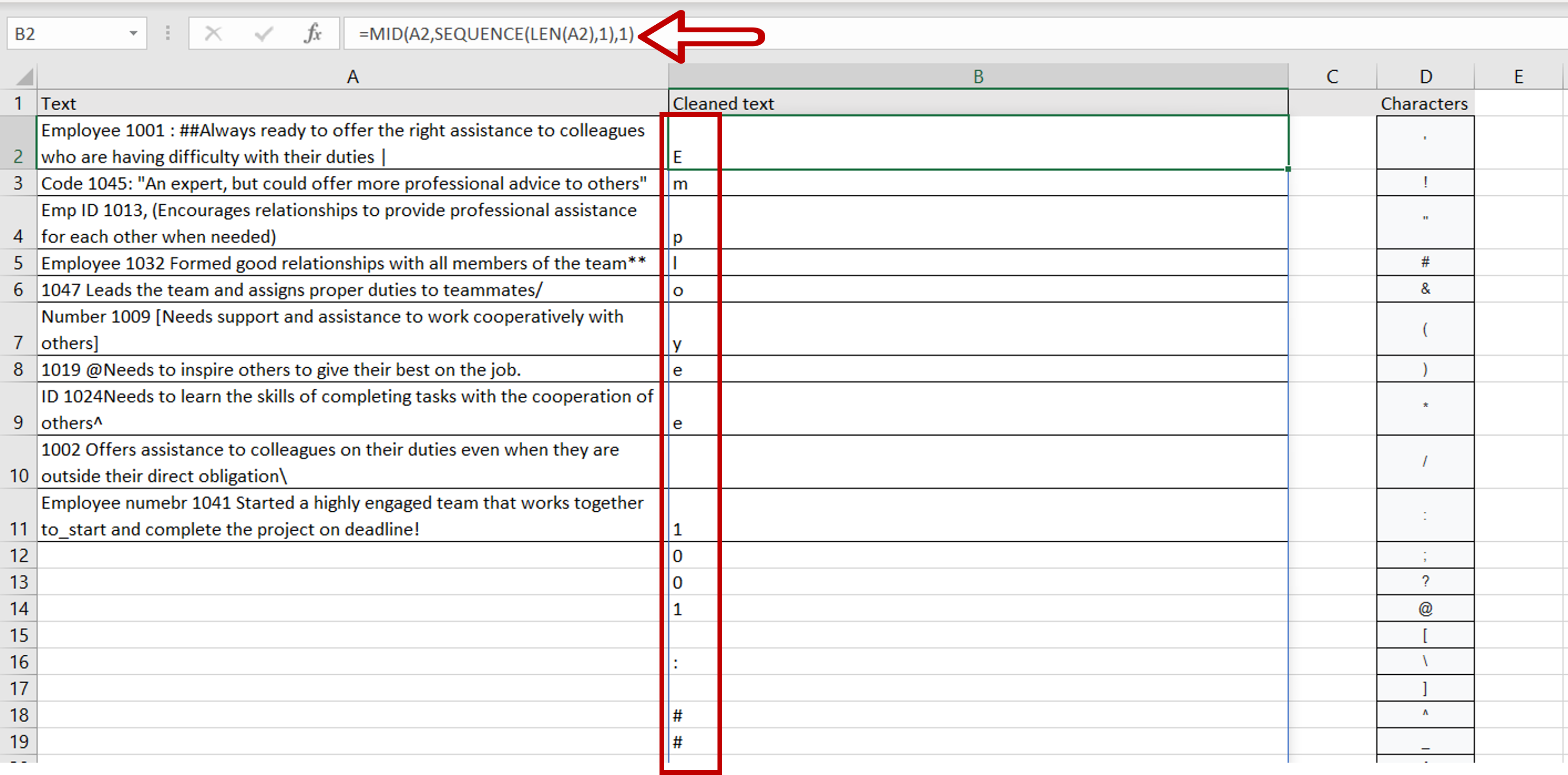
– Select the cell with the formula
– Enhance the formula with the MID() function
= MID(Text,SEQUENCE(LEN(Text),1),1)
– Press Enter
– The MID() function is used with the array so the number of characters to be returned is 1 for each character in the array
Step 4 – Remove the special characters
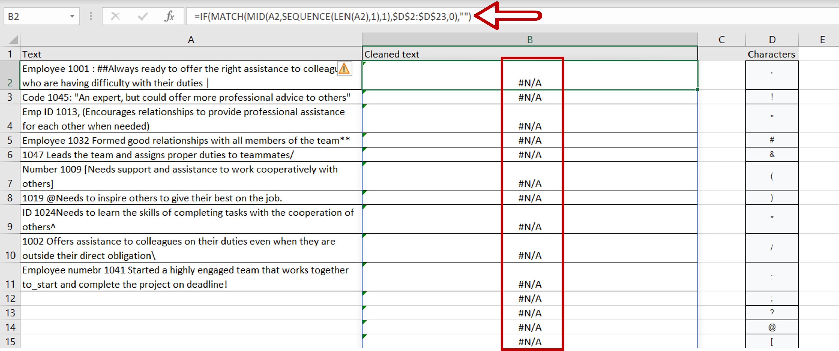
– Select the cell with the formula
– Enhance the formula with the MATCH() and IF() functions
=IF(MATCH(MID(Text,SEQUENCE(LEN(Text),1),1),$range of Characters$,0),””)
– Press Enter
– The MATCH() function looks for each value in the array in the lookup table of characters and returns the position of the character as a number
– The range of characters is made constant by selecting the cell reference and pressing F4
– Characters not in the lookup table are replaced by an error value
– The IF() function replaces the number with nothing, signified by the double quotes (“”)
Step 5 – Replace the errors with actual values
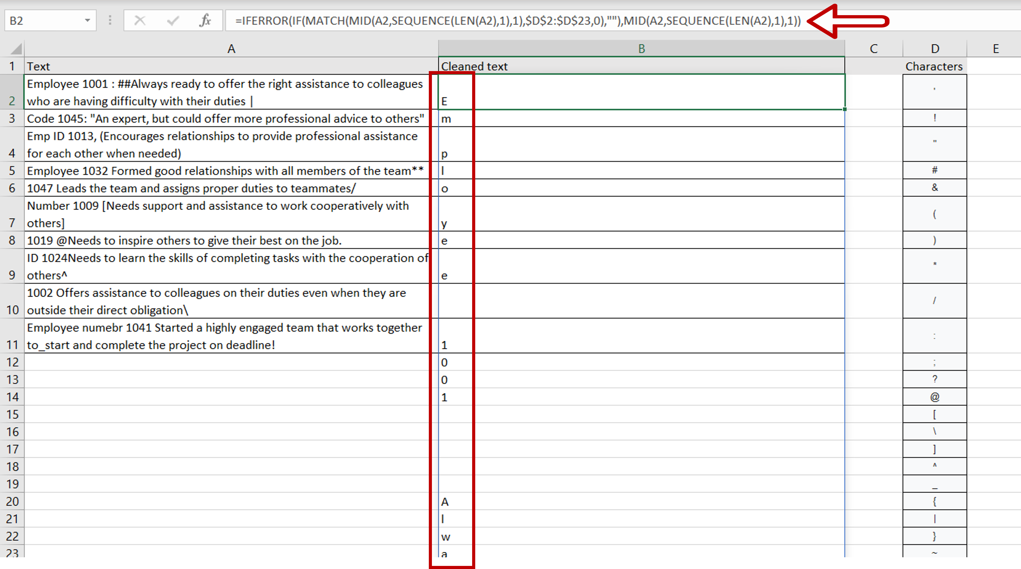
– Select the cell with the formula
– Enhance the formula with the IFERROR() function
=IFERROR(IF(MATCH(MID(Text,SEQUENCE(LEN(Text),1),1),$range of Characters$,0),””),MID(Text,SEQUENCE(LEN(Text),1),1))
– Press Enter
– The errors are replaced by the actual values
Step 6 – Collapse the array into a single string
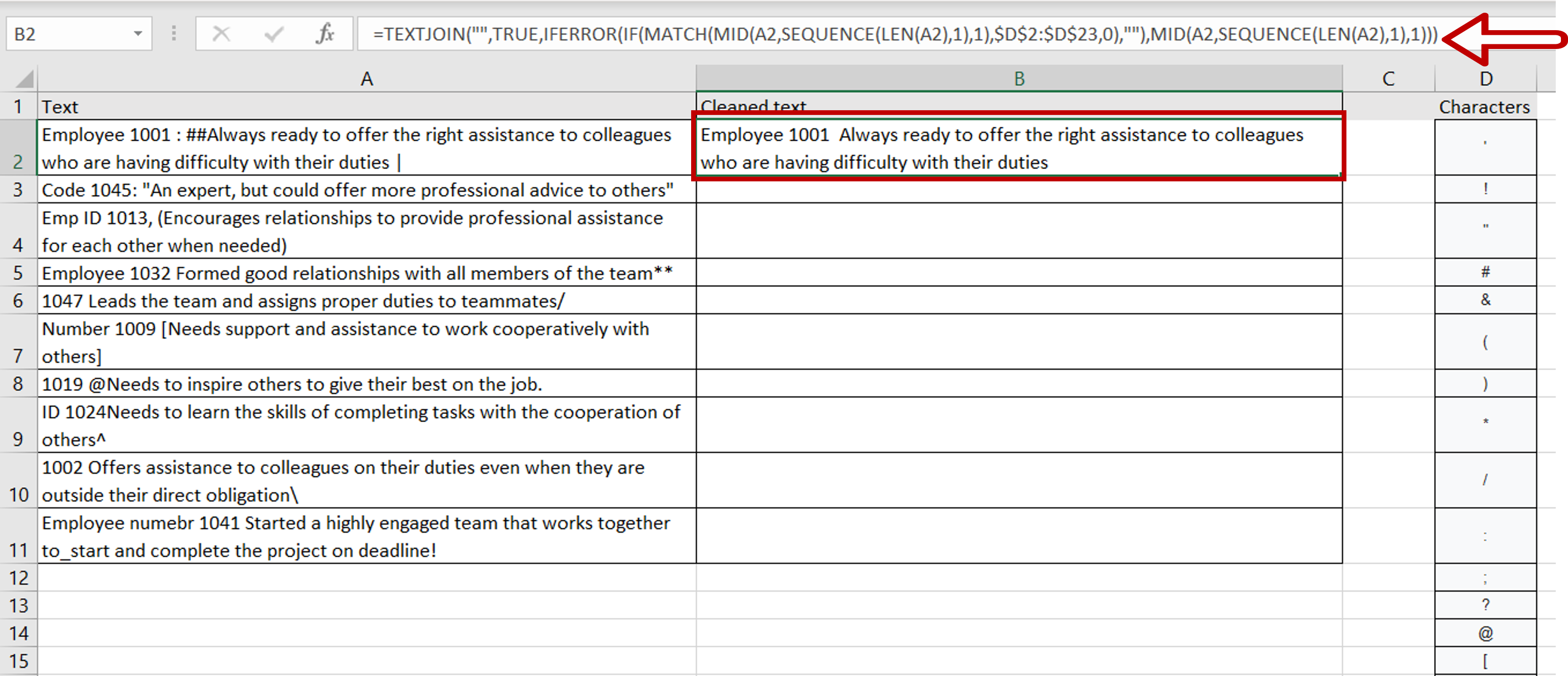
– Select the cell with the formula
– Enhance the formula with the TEXTJOIN() function
=TEXTJOIN(“”,TRUE, IFERROR(IF(MATCH(MID(Text,SEQUENCE(LEN(Text),1),1),$range of Characters$,0),””),MID(Text,SEQUENCE(LEN(Text),1),1)))
– Press Enter
– No delimiter is used (“”) and the value TRUE tells the function to ignore empty cells
Step 7 – Copy the formula
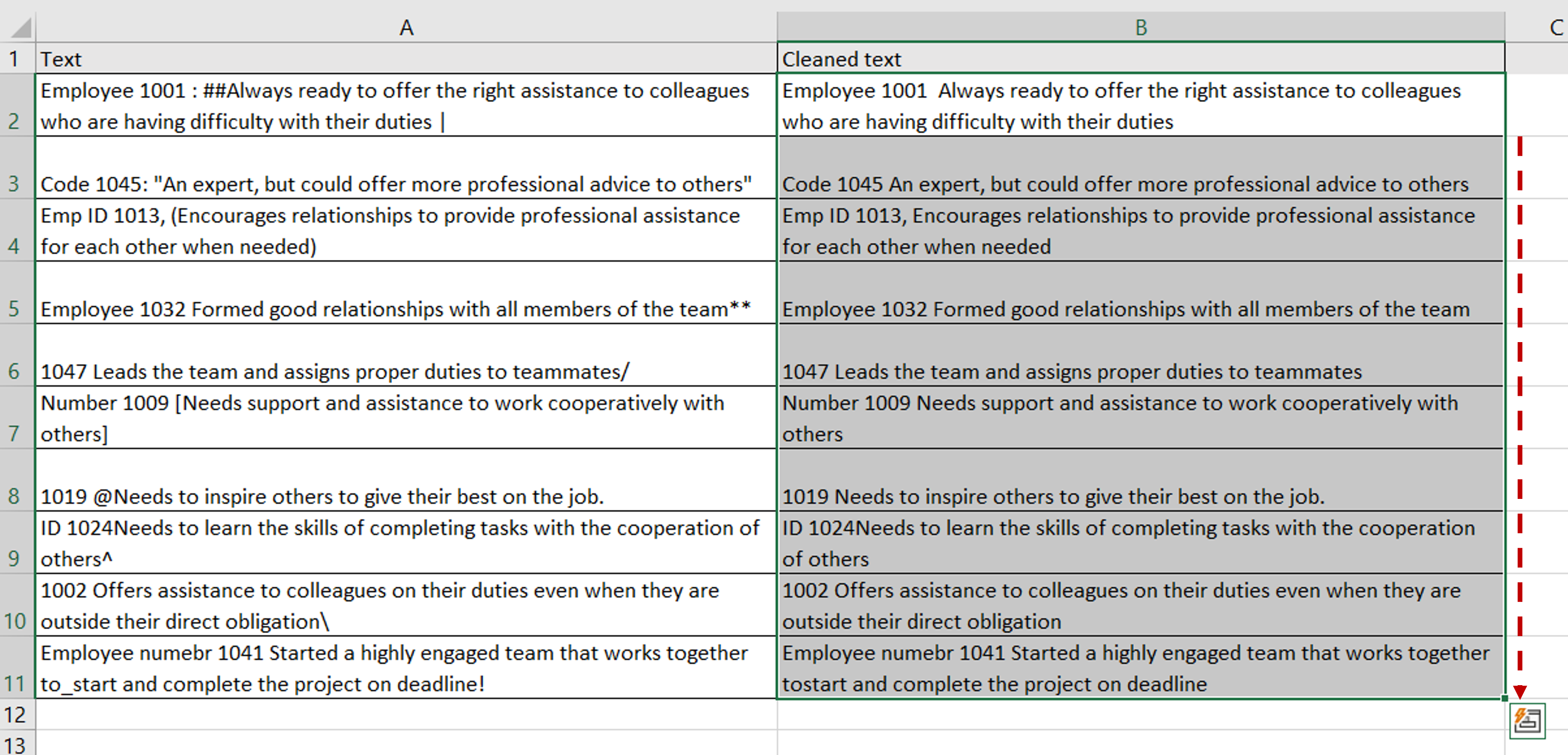
– Using the fill handle from the first cell, drag the formula to the remaining cells
OR
a) Select the cell with the formula and press Ctrl+C or choose Copy from the context menu (right-click)
b) Select the rest of the cells in the column and press Ctrl+V or choose Paste from the context menu (right-click)
Step 8 – Check the result
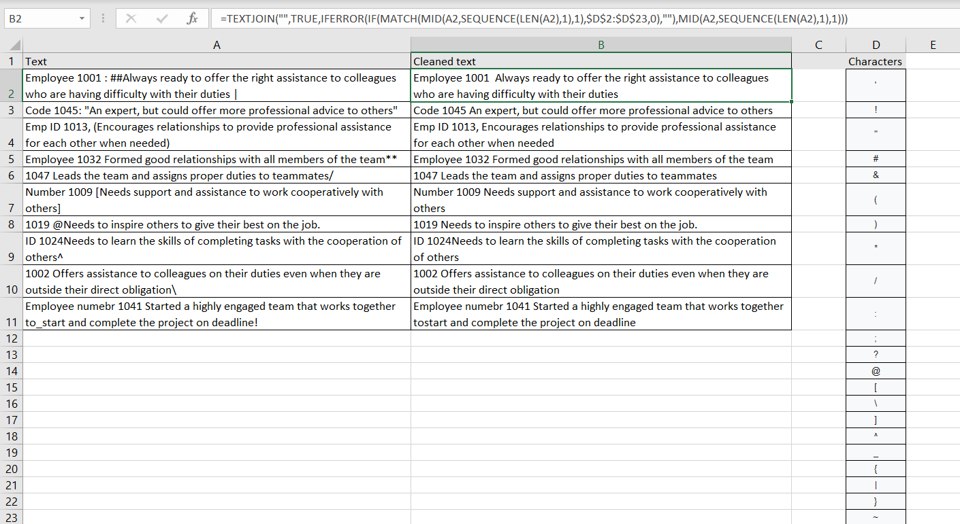
– The special characters given in the ‘Characters’ lookup table are removed from the text in each row


