
How to remove non-numeric characters from cells in Excel
 By
SpreadCheaters
By
SpreadCheaters
You can watch a video tutorial here.
Excel has many features and tools to help with formatting and manipulating text and numbers in cells. When cleaning up data or performing data analysis, you may need to remove all the non-numeric characters from a cell or cells. This amounts to extracting only the numeric characters from the cells. This happens many times when analyzing or cleaning textual data such as customer feedback or transcripts.
In this example, we will look at a transcript of employee appraisals. The employee code is part of the transcript and needs to be extracted to a separate column so that it can be stored along with the text of the transcript. The approach to building the formula works is explained below:
1. Create an array of numbers equal to the length of the text in the cell using the ROW() and INDIRECT() functions
a. ROW() function: this returns the row number of the cell reference
i. Syntax: ROW(cell reference)
1. cell reference: (optional)the reference of the cell for which you want the row number. If this is left blank, it takes the row number of the cell it is in
b. INDIRECT() function: this returns the reference given by a string. Here it is used to transform the values returned by ROW() into an array
i. Syntax: INDIRECT(reference)
1. reference: the cell that contains the reference
2. Put each character in the text into the array using the MID() function
a. MID() function: this returns a specified number of characters from a string
i. Syntax: MID(text, start number, number of characters)
1. text: the string from which the characters are to be extracted
2. start number: the number of the character from which the extraction is to start
3. number of characters: the number of characters to extract
3. Multiply the array by 1 to convert non-numeric characters into errors and keep numeric characters as they are
4. Replace the errors with blank spaces using the IFERROR() function.
a. IFERROR() function: if a formula results in an error, this function replaces the error with a specified value
i. Syntax: IFERROR(formula,value)
1. formula: the formula to be evaluated
2. value: the value to be returned if the formula returns an error
5. Collapse the array into a single string using the TEXTJOIN() function
a. TEXTJOIN() function: this combines multiple pieces of text into a single string using the specified delimiter
i. Syntax: TEXTJOIN(delimiter, ignore_empty, text1, text 2…….)
1. delimiter: the delimiter to be used between the pieces of text
2. ignore_empty: if set to TRUE, this ignores empty pieces of text
3. text1, text 2…..: the pieces of text to be joined. At least one piece is mandatory
Note: In some versions of Excel, this formula is to be treated as an array formula. After creating the entire formula, press Ctrl+Shift+Enter instead of just Enter.
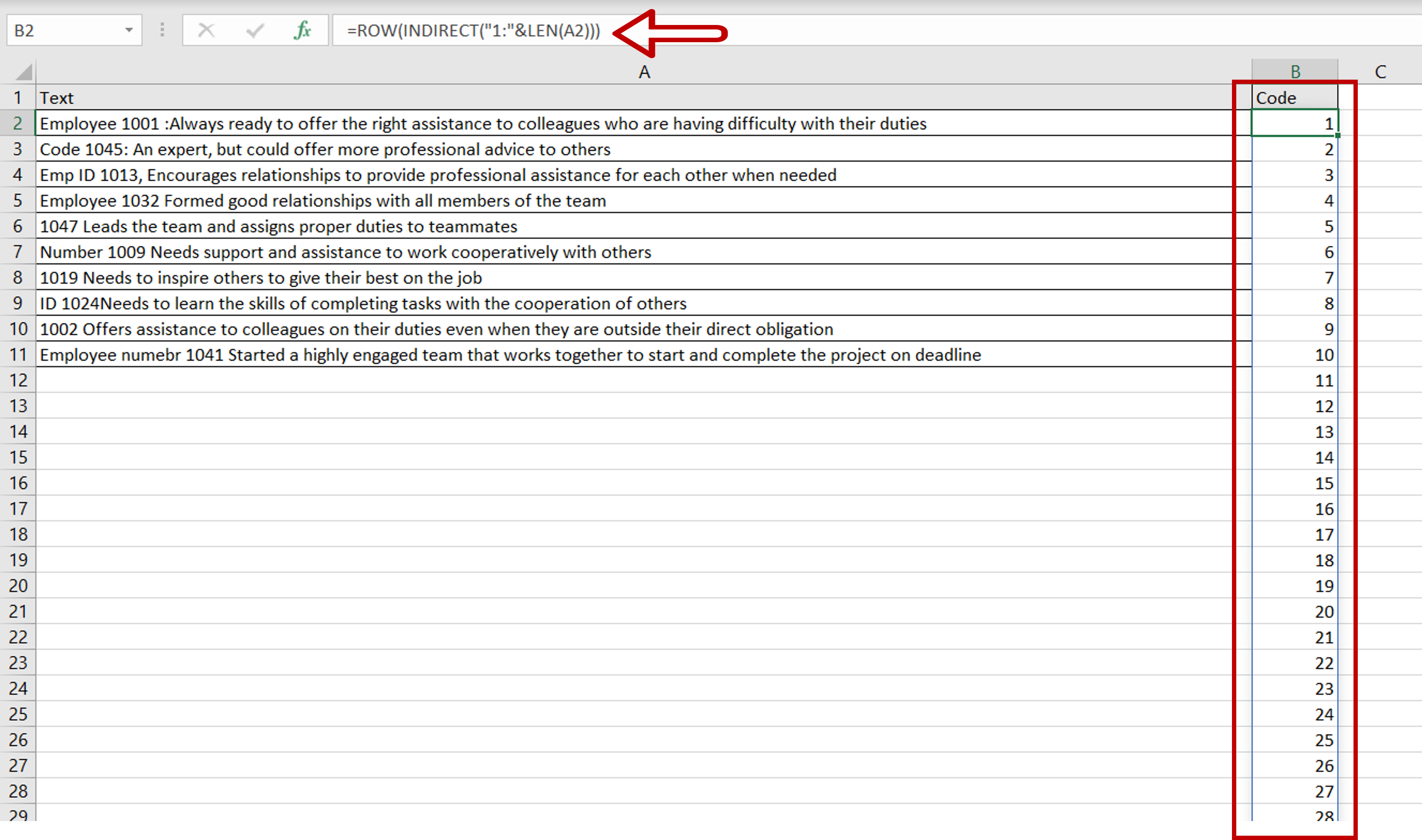
Step 1 – Create the array of numbers
– Select the cell in which the result is to be displayed
– Type the formula using cell references:
=ROW(INDIRECT(“1:”&LEN(Text)))
– Press Enter
This creates an array of numbers equal to the length of the text
Note: If you encounter a #SPILL! error then it means that the rows below the selected cell contain data and the array cannot be displayed. Remove the data in the cells below to see the array.
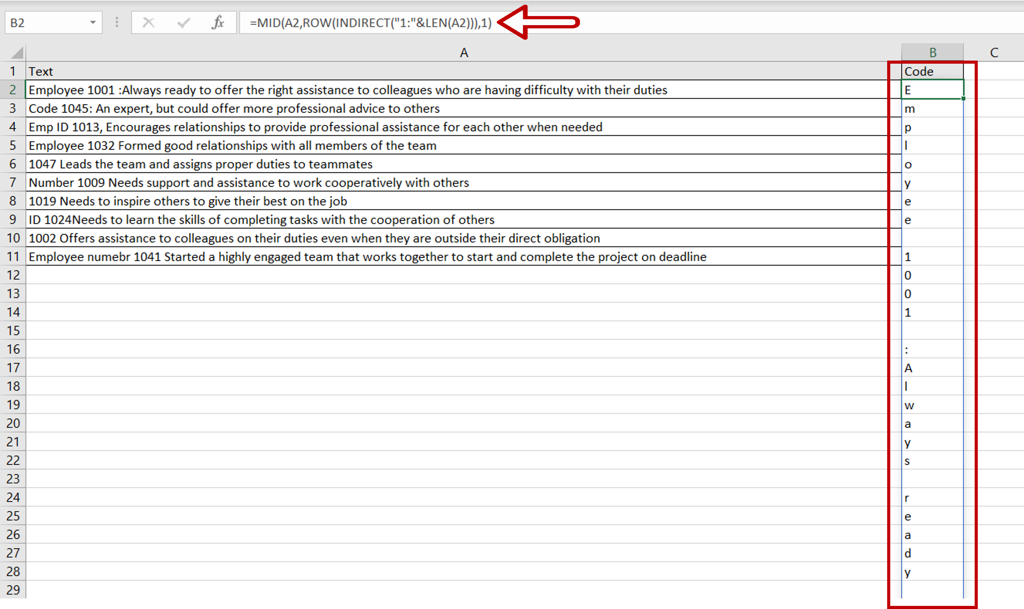
Step 2 – Add each character to the array
– Select the cell with the formula
– Enhance the formula with the MID() function
=MID(Text,ROW(INDIRECT(“1:”&LEN(Text))),1)
– Press Enter
The MID() function is used with the array so the number of characters to be returned is 1 for each character in the array
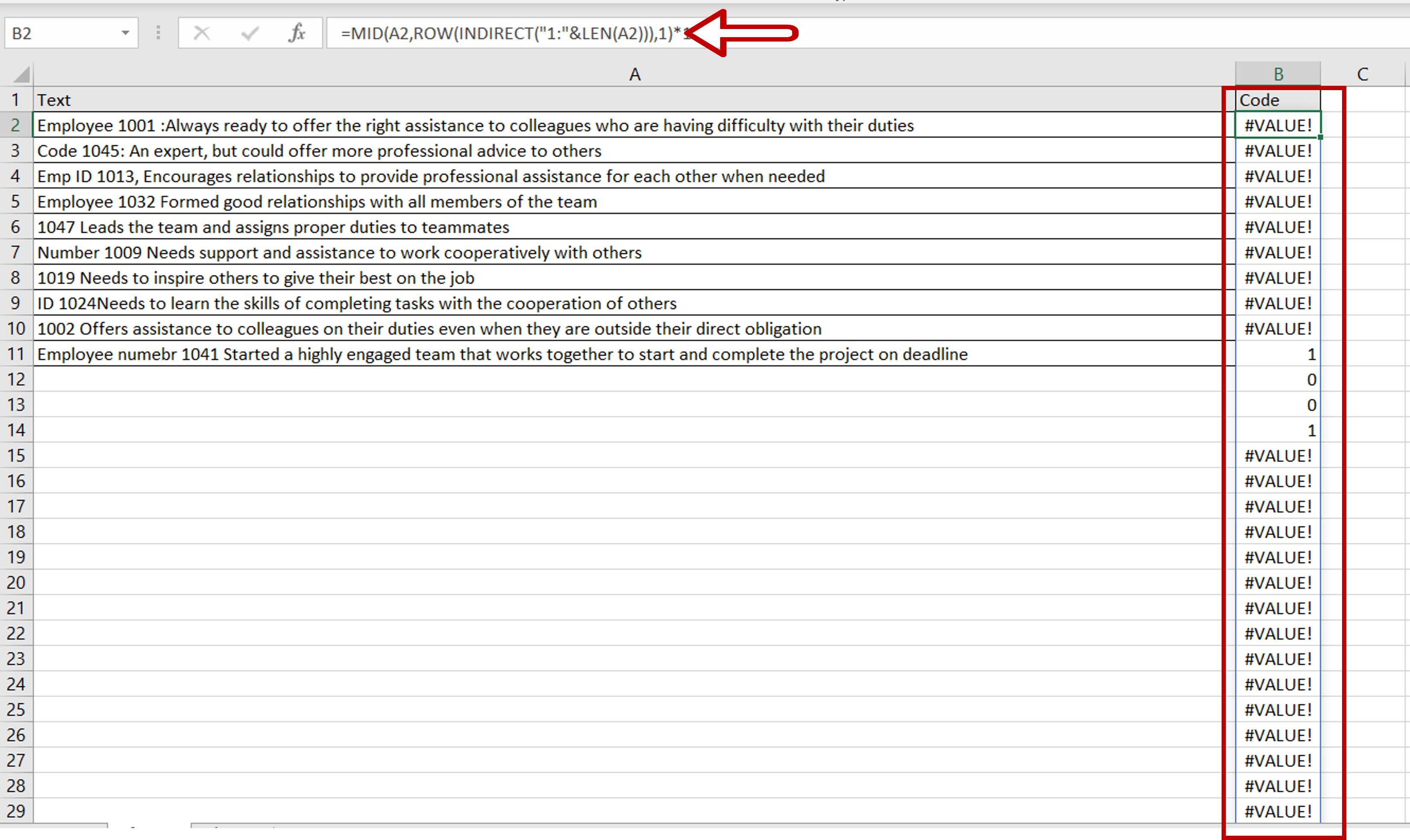
Step 3 – Multiply the array by 1
– Select the cell with the formula
– Enhance the formula by adding ‘*1’
=MID(Text,ROW(INDIRECT(“1:”&LEN(Text))),1)*1
– Press Enter
– Non-numeric characters are replaced by an error value
Step 4 – Replace the errors with blanks
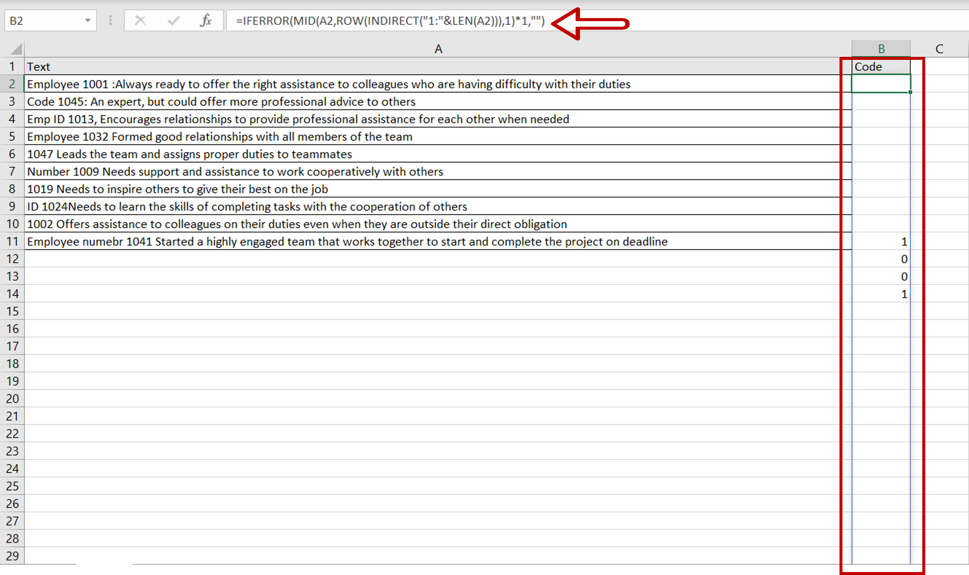
– Select the cell with the formula
– Enhance the formula with the IFERROR()
function
=IFERROR(MID(Text,ROW(INDIRECT(“1:”&LEN(Text))),1)*1,””)
– Press Enter
– The errors are replaced by empty values
Step 5 – Collapse the array into a single string
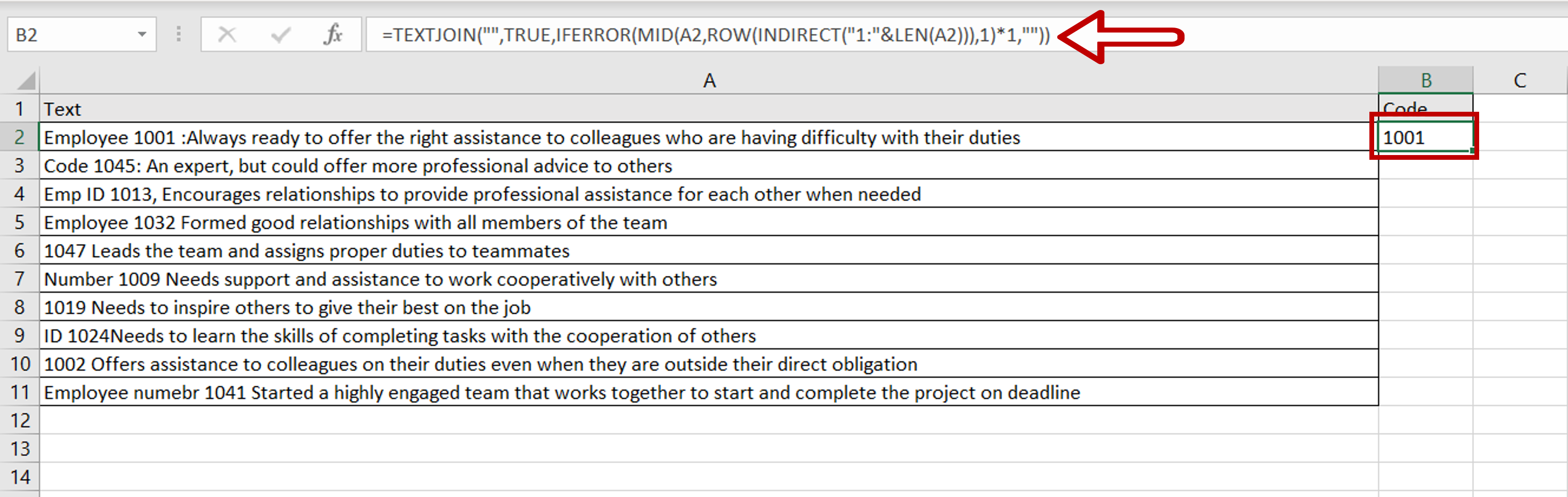
– Select the cell with the formula
– Enhance the formula with the TEXTJOIN() function
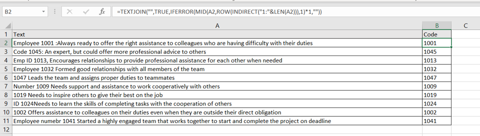
=TEXTJOIN(“”,TRUE,IFERROR(MID(Text,ROW(INDIRECT(“1:”&LEN(Text))),1)*1,””))
– Press Enter
– No delimiter is used (“”) and the value TRUE tells the function to ignore empty cells
Step 6 – Copy the formula
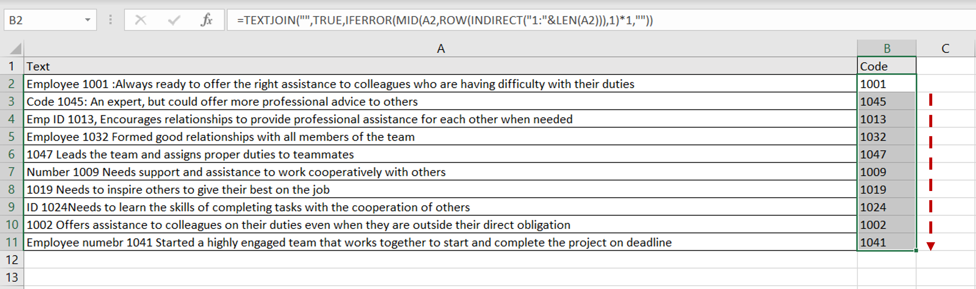
– Using the fill handle from the first cell, drag the formula to the remaining cells
OR
a) Select the cell with the formula and press Ctrl+C or choose Copy from the context menu (right-click)
b) Select the rest of the cells in the column and press Ctrl+V or choose Paste from the context menu (right-click)
Step 7 – Check the result

– The non-numeric characters are removed from the text in each row and only the numeric characters, in this case, the employee code, are returned


