How to remove negative sign in Microsoft Excel

Excel is a widely used spreadsheet software that allows users to manage, organize, and analyze data in a tabular format. Developed by Microsoft, Excel provides a range of features and tools, including functions, formulas, charts, tables, and pivot tables, to help users perform complex calculations, create visualizations, and gain insights from their data. 

In this tutorial we will learn how to remove negative signs in Microsoft Excel.In Excel, negative signs can be removed from numeric values using various methods. One of the easiest ways is to use the ABS (absolute) function, which converts negative numbers into positive numbers.We can also use IF function to remove negative sign in excel.

Method 1 : Using ABS function to Remove Negative Sign

Step 1 – Select a Blank Cell

• Select  a blank cell where you want to remove the negative sign.

Step 2 – Place  an Equals Sign

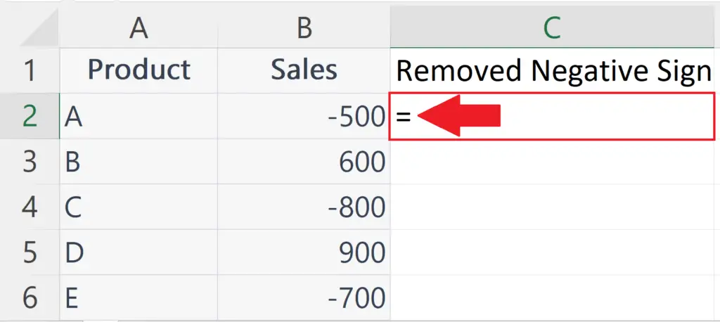
• Place an Equals sign in the blank cell.

Step 3 – Use the ABS function

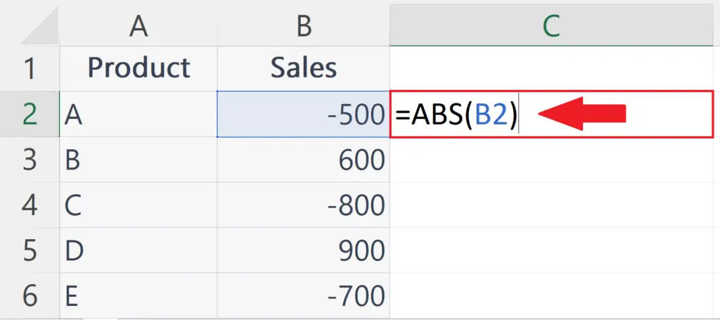
• The ABS function is a mathematical function in Excel that returns the absolute value of a number, which is the value of the number without its sign. In other words, the ABS function converts negative numbers into positive numbers, and leaves positive numbers unchanged.
• The syntax of the ABS function is : 

                                   ABS(A2)

• Where  the argument A2 is the address of the cell containing the number whose sign is to be removed.

Step 4 – Press the Enter Key

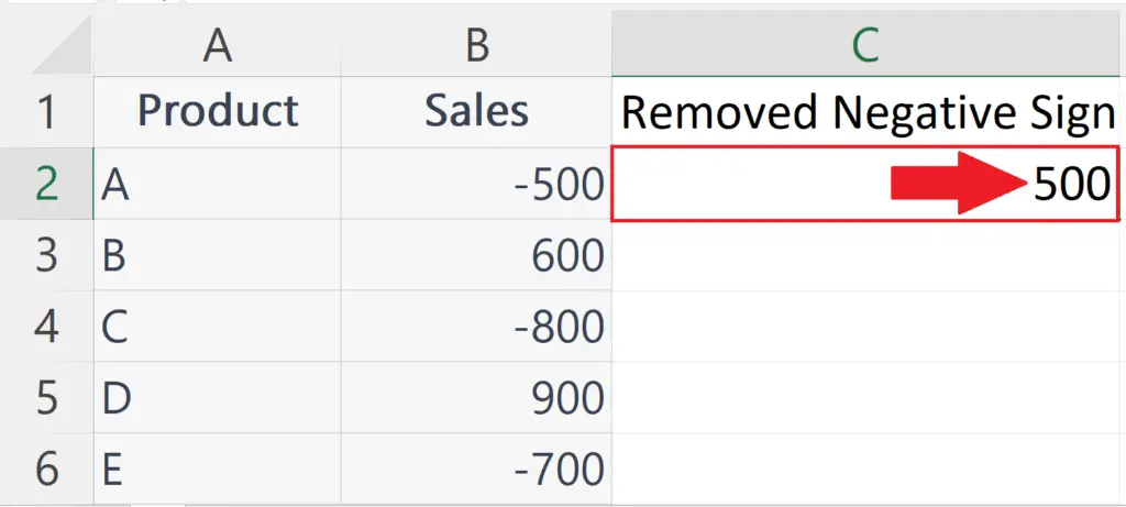
• Press the Enter key to remove the negative sign.

Step 5 – Remove the Negative Sign from all the data

• To remove the negative sign from all the data set use the “Handle Select” and “Drag and Drop” method to apply ABS function to all the data.

Method 2 : Using IF Function to Remove the Negative Signs

Step 1 – Select a Blank Cell

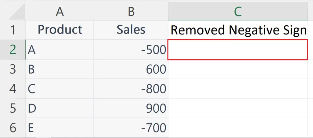
• Select  a blank cell where you want to remove the negative sign.

Step 2 – Place  an Equals Sign

• Place an Equals sign in the blank cell.

Step 3 – Use IF function

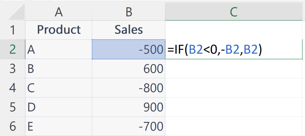
• The syntax for the formula made by IF function will be:

                                                IF(A2<0,-A2,A2)

• Where the first argument A2<0 is the logical test.
• Second argument i.e. -A2 is the value that the function will return if the condition is TRUE.The function will reverse the sign of the number in cell A2 if the number is smaller than 0 (negative).
• The third argument i.e. A2 is the value that the function will return if the condition is False.The function will leave the number as it is if the number is greater than or equal to zero (positive).

Step 4 – Press the Enter Key

• Press the Enter key to remove the negative sign.

Step 5 – Remove the Negative Sign from all the data

• To remove the negative sign from all the data set, use the “Handle Select” and “Drag and Drop” method to apply the formula  to all the data set.