
How to remove #n/a in Excel
 By
SpreadCheaters
By
SpreadCheaters
You can watch a video tutorial here.
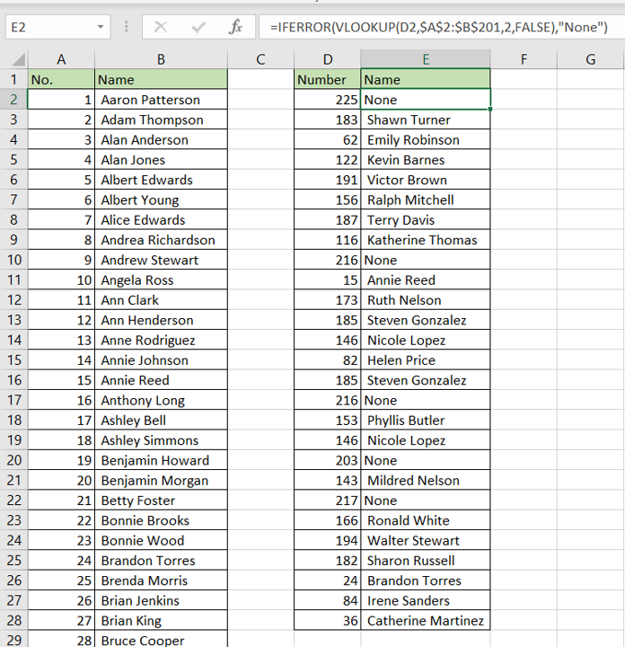
The #N/A error occurs in Excel when a value is not available. This error is displayed when a formula or function cannot find what it is looking for. While this does alert you to a possible mistake such as not making a cell reference constant when copying a formula, there are cases when this is a result of a function behaving correctly. The most common example is when using the VLOOKUP function. When the VLOOKUP function finds a match, it returns the match and if it does not, it returns the #N/A error. Although this is not exactly an error, the #N/A displayed in the cell gives the impression that the function has not worked correctly.
The IFERROR() function can be used to remove or suppress the #N/A error:
1. IFERROR() function: if a formula results in an error, this function replaces the error with a specified value
a. Syntax: IFERROR(formula,value)
i. formula: the formula to be evaluated
ii. value: the value to be returned if the formula returns an error
Step 1 – Edit the cell
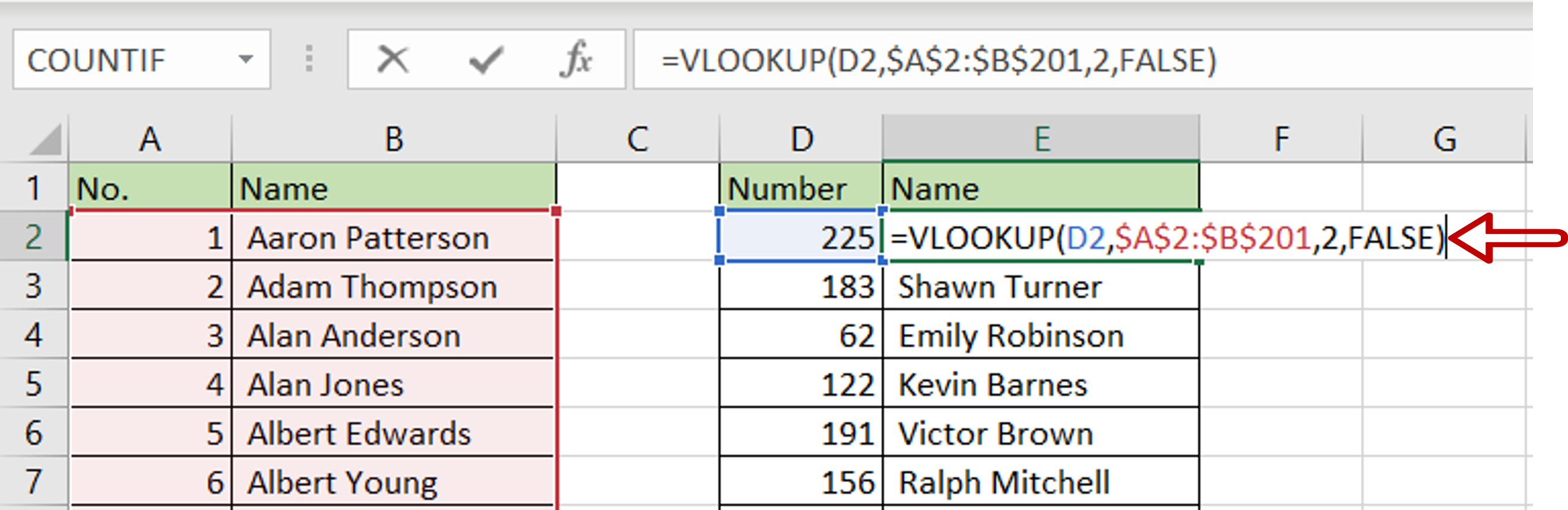
– Select the first cell with the VLOOKUP formula
– Press F2 or click the formula bar to edit the formula
Step 2 – Add the IFERROR() function
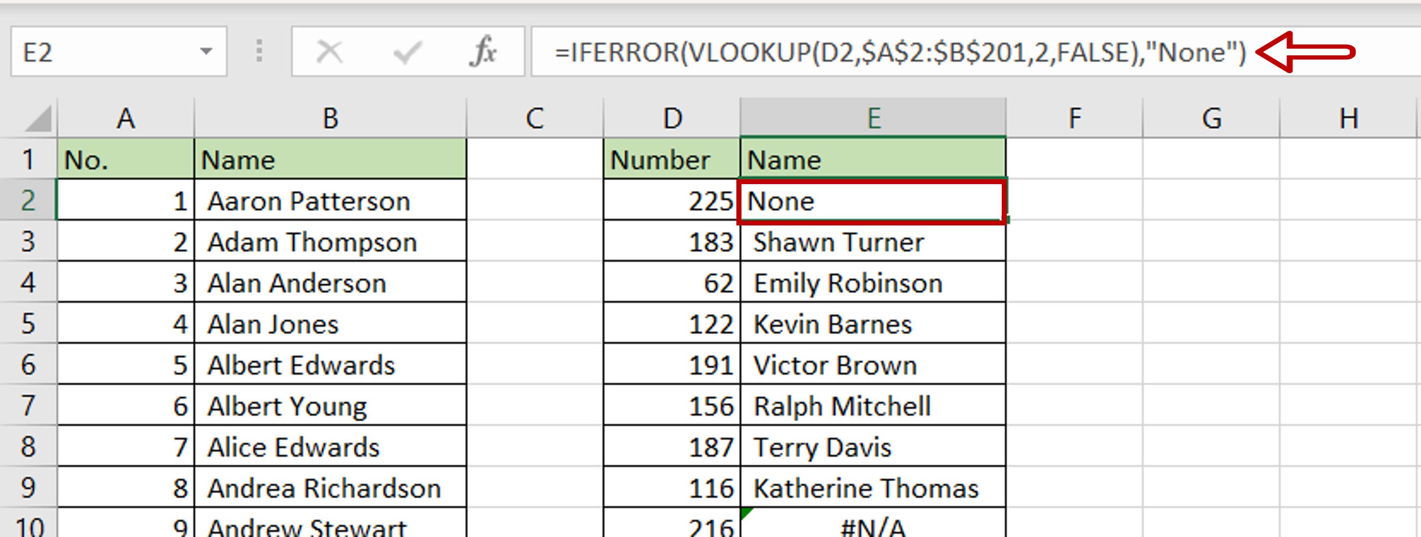
– Edit the formula as:
=IFERROR(VLOOKUP formula, “None”)
– The IFERROR function inserts the value “None” if the value is not available
– Press Enter
Step 3 – Copy the formula
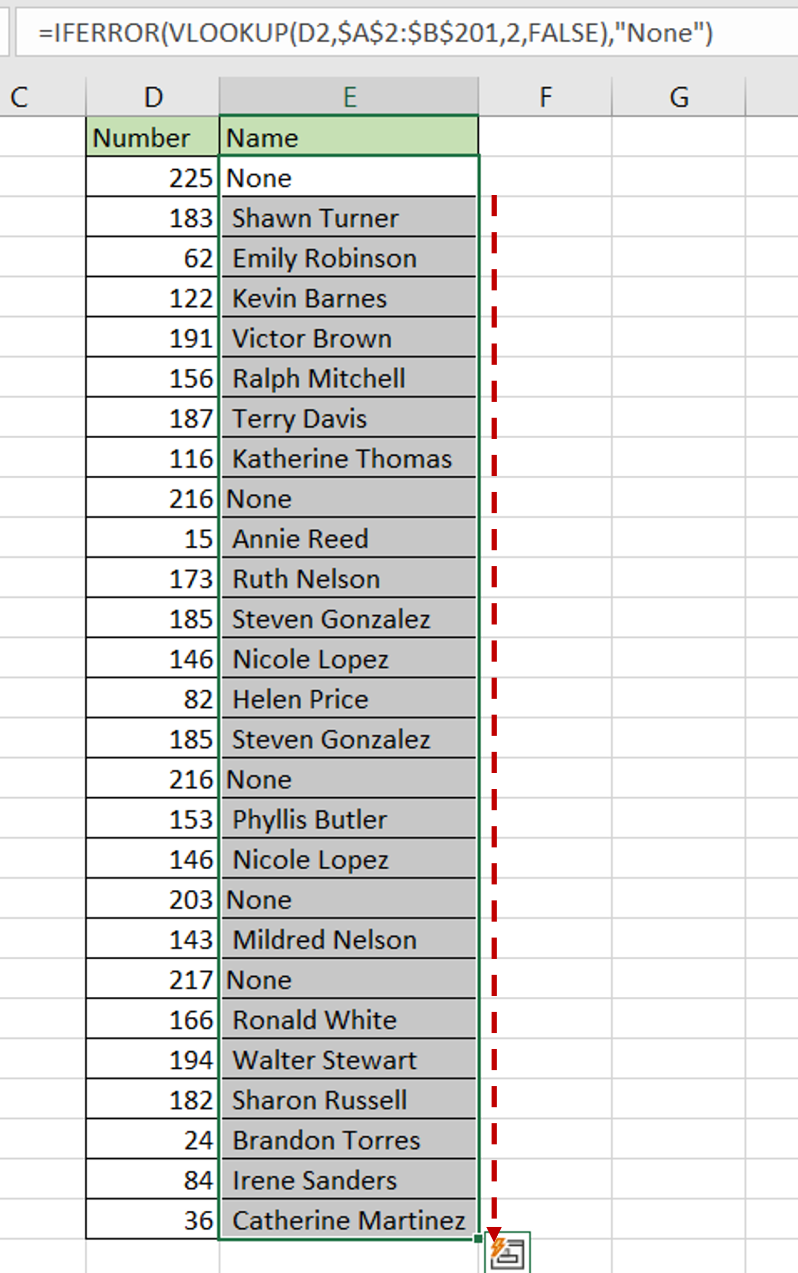
– Using the fill handle from the first cell, drag the formula to the remaining cells
OR
a. Select the cell with the formula and press Ctrl+C or choose Copy from the context menu (right-click)
b. Select the rest of the cells in the column and press Ctrl+V or choose Paste from the context menu (right-click)
Step 4 – Check the result
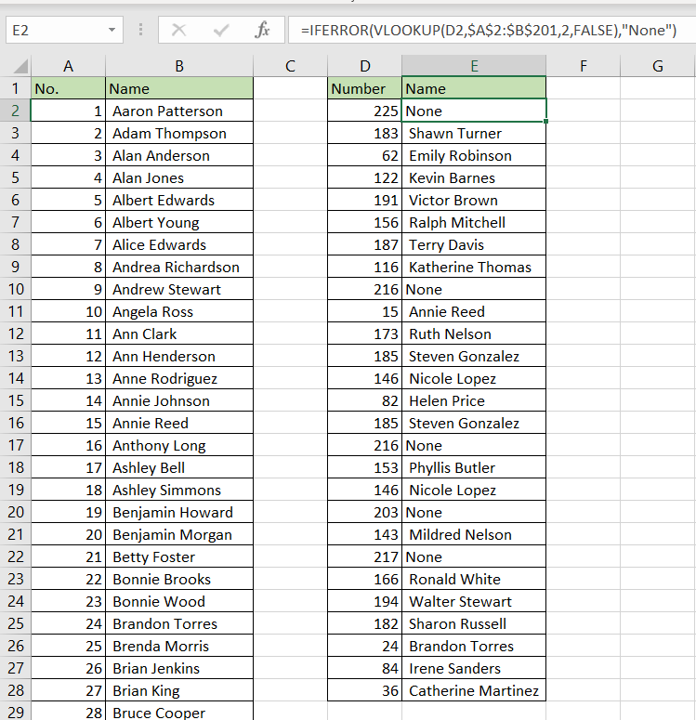
– Wherever VLOOKUP cannot find a match, the word “None” is inserted into the cell
– The #N/A error is removed


