How to remove gridlines in Excel for specific cells

You can watch a video tutorial here.

As a spreadsheet application, the workspace in Excel displays a grid of cells in the form of rows and columns. By default, the gridlines are visible but they can be removed from the display. The setting not to display the gridlines applies to the entire sheet and cannot be applied to specific cells. When formatting a sheet, you may want to remove the gridlines for specific cells to make the information in those cells stand out. Here we will look at using workarounds to suppress the display of gridlines for specific cells.

Option 1 – Change the color of the cell border 

Step 1 – Select the area

• Select the area for which the gridlines are to be removed

Step 2- Open the Format Cells window

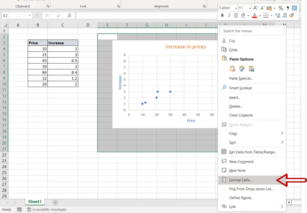
• Right-click and select Format Cells  from the context menu

OR

Go to Home > Number  and click on the arrow to expand the menu

OR

Go to Home > Cells > Format > Format Cells

OR

Press Ctrl+1

Step 3 – Change the color of the border

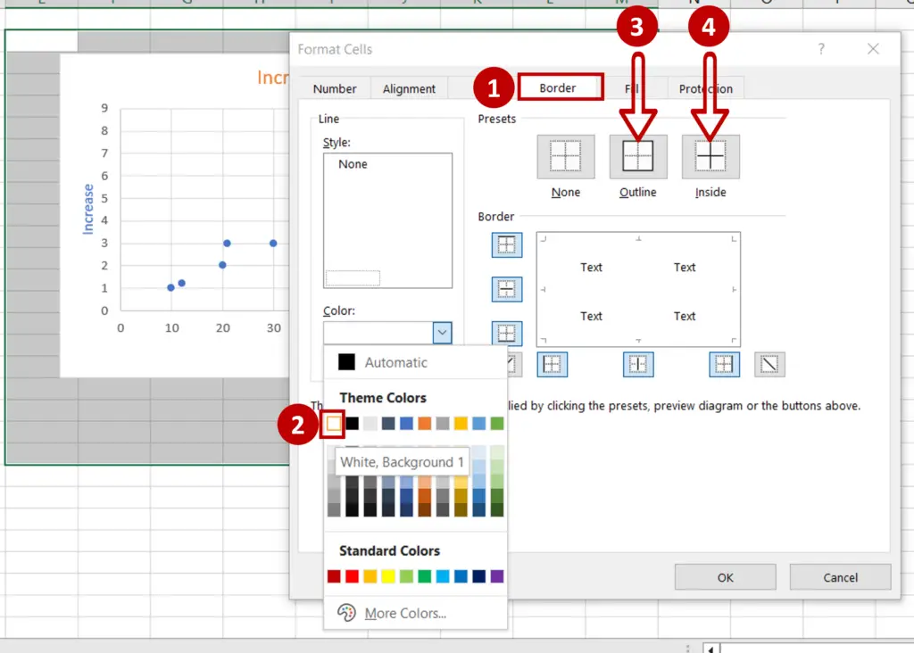
• Go to the Border tab 
• Select the Color as ‘White, Background 1’
• Click on the Outline button
• Click on the Inside button
• Click OK

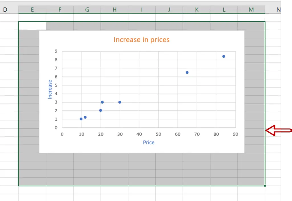
Step 4 – Check the result

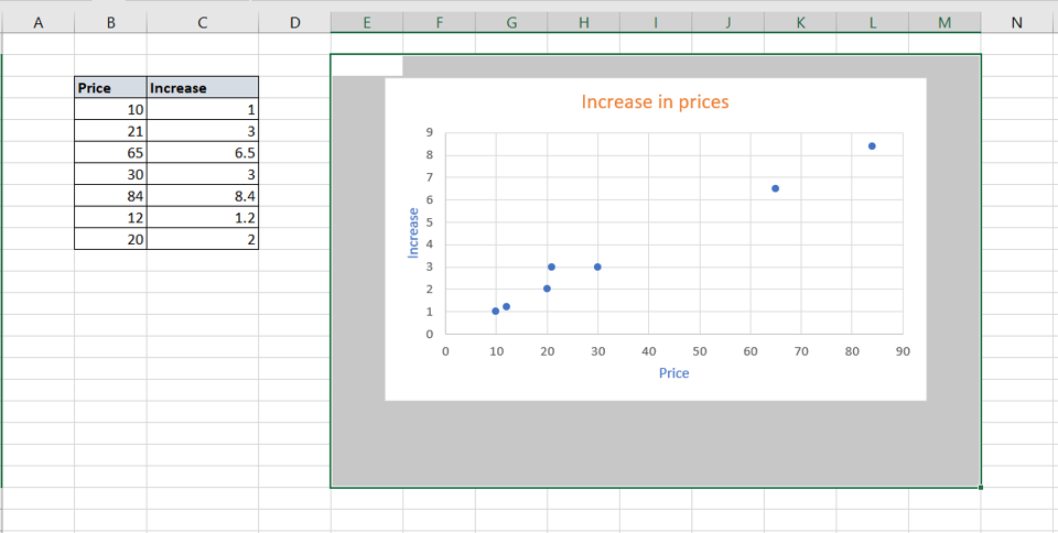
• The cell border color is changed to white so the gridlines are not visible

Option 2 – Change the background color of the cell 

Step 1 – Select the area

• Select the area for which the gridlines are to be removed

Step 2- Open the Format Cells window

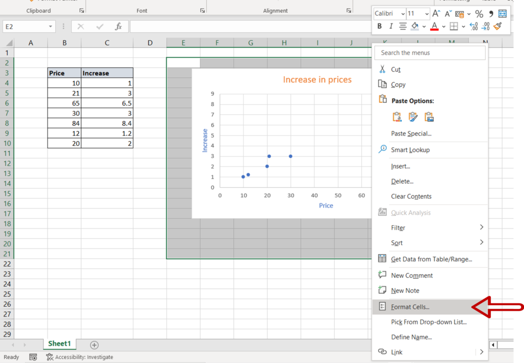
• Right-click and select Format Cells  from the context menu

OR

Go to Home > Number  and click on the arrow to expand the menu

OR

Go to Home > Cells > Format > Format Cells

OR

Press Ctrl+1

Step 3 – Change the background color of the cell

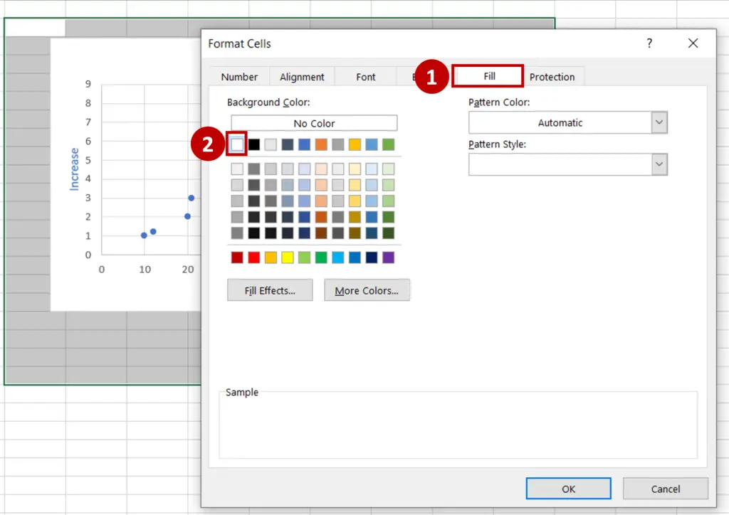
• Go to the Fill tab 
• Select white as the Background Color 
• Click OK

Step 4 – Check the result

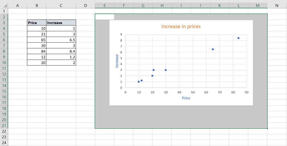
• The background color of the cell is changed to white so the gridlines are not visible