How to rank in Excel from highest to lowest
You can watch a video tutorial here.
Excel is popular as a spreadsheet application but is also frequently used as a database and to create lists. Very often, when you are looking at a set of data, you would be interested in knowing the rank or position of each row with respect to a particular value. For example, you need to find the top ten branches in terms of sales.
In Excel, there are 2 ways of doing this:
- Sort the data
- RANK() function: this gives the rank of a number in a list of numbers
- Syntax: RANK(number, reference, order)
- number: the number to which the rank is to be assigned
- reference: the list of numbers in which the number is to be ranked
- order: (optional) this specifies whether the numbers are to be considered in ascending or descending order
Option 1 – Sort the data
Step 1 – Select the data

- Select the data to be ranked
Step 2 – Open the Sort box
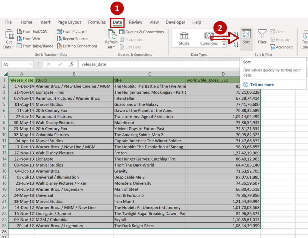
- Go to Data > Sort & Filter
- Click on the Sort button
Step 3 – Set the parameters
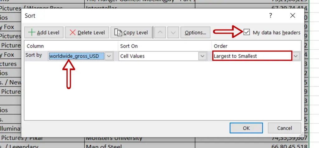
- Tick My data has headers
- Define the parameters for the sort
- Sort by: ‘worldwide_gross_USD’
- Order: Largest to Smallest
- Click OK
Step 4 – Insert a column

- Select Column A
- Right-click and choose Insert from the context menu
Step 5 – Create the ranks

- Name the new column ‘Rank’
- Type the first 2 numbers of the rank sequence i.e. 1,2
- Select the numbers and drag the fill handle down to the end of the data
Step 6 – Check the result

- The rows are now ranked from highest to lowest in terms of ‘worldwide_grosss_USD’
Option 2 – Use the RANK() function
Step 1 – Create the formula

- Select the cell in which the rank is to be displayed
- Type the formula using cell references:
=RANK(worldwide_gross_USD, range of worldwide_gross_USD)
- Press Enter
Step 2 – Copy the formula

- Using the fill handle from the first cell, drag the formula to the remaining cells
OR
- Select the cell with the formula and press Ctrl+C or choose Copy from the context menu (right-click)
- Select the rest of the cells in the column and press Ctrl+V or choose Paste from the context menu (right-click)
Step 3 – Open the Sort box
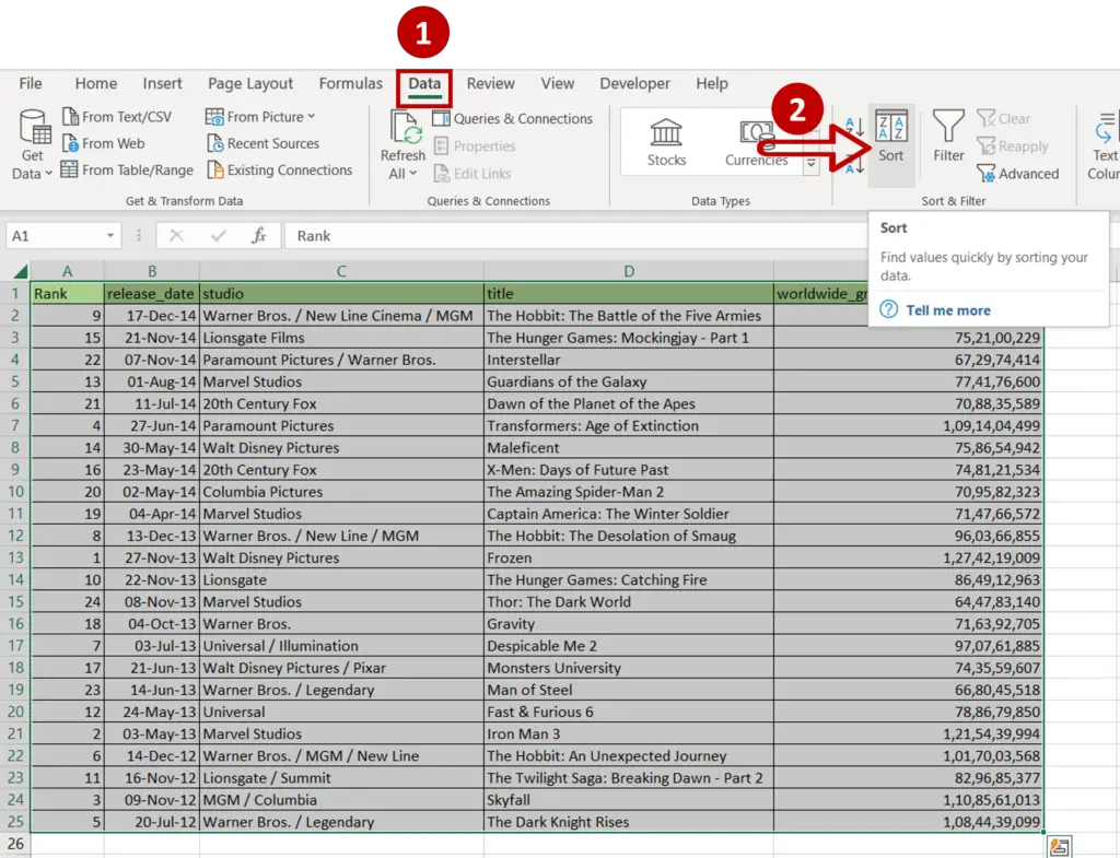
- Select the data
- Go to Data > Sort & Filter
- Click on the Sort button
Step 4 – Set the parameters
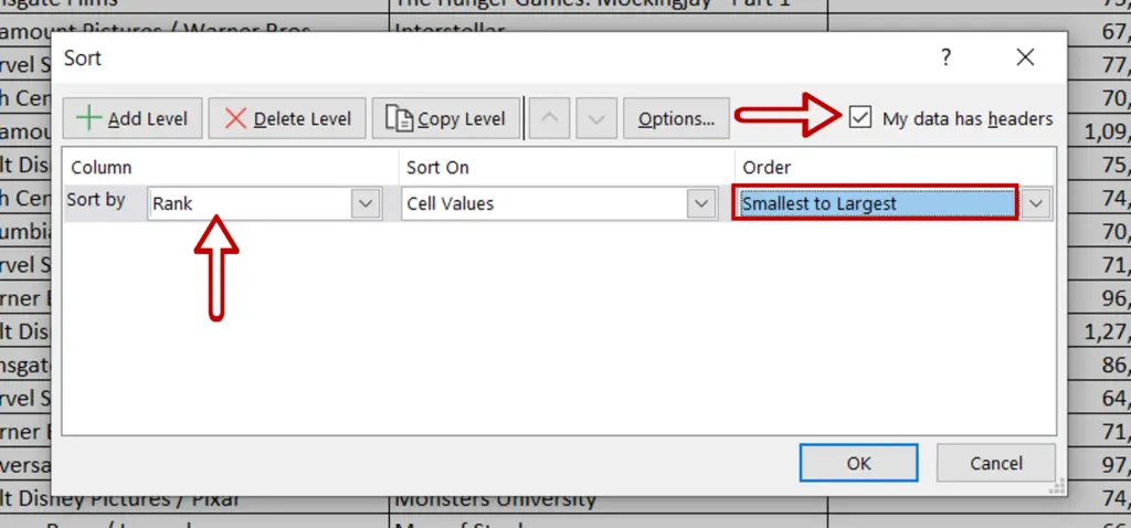
- Tick My data has headers
- Define the parameters for the sort
- Sort by: ‘Rank’
- Order: Smallest to Largest
- Click OK
Step 5 – Check the result

- The rows are now ranked from highest to lowest in terms of ‘worldwide_grosss_USD’


