How To Randomly Select Rows In Excel

Have you ever needed to randomly select rows from a large dataset in Excel? Whether you’re conducting a survey, analyzing data, or simply shuffling rows for a randomized order, Excel provides several methods to accomplish this task. In this article, we’ll explore various techniques to help you efficiently and randomly select rows in Excel, allowing you to work with a subset of data that meets your specific requirements.

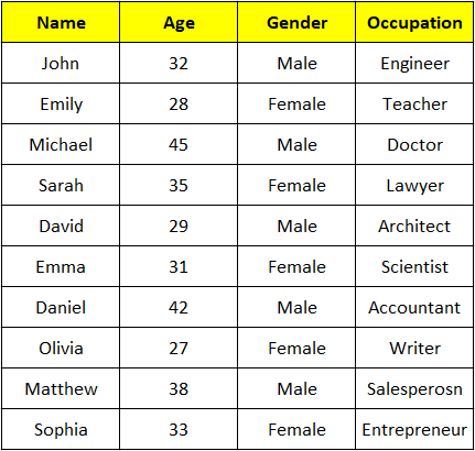
We will be using this dataset for today’s article.

Method 1 – Using RAND Function

The RAND function in Excel is a built-in function that generates a random decimal number between 0 and 1. It’s a volatile function, meaning that it recalculates every time there is a change in the worksheet, ensuring that the generated random number is always up-to-date.

The syntax for the RAND function is simple:

=RAND()

RAND: This is the name of the function in Excel that generates random numbers.

(): These parentheses are used to enclose any arguments that the function may require. In the case of the RAND function, there are no arguments, so the parentheses are left empty.

Step 1 – Select The Cell 

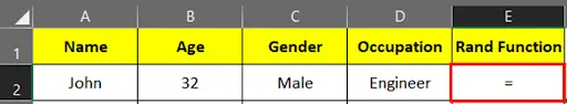
• Select the cell where you want to have random numbers, starting with equals (=) to sign.

Step 2 – Type The Formula

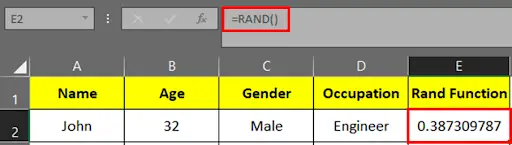
• In cell E2 enter the following formula: =RAND(). This formula generates a random number between 0 and 1 for each row and press enter.

Step 3 – Copy The Formula Down

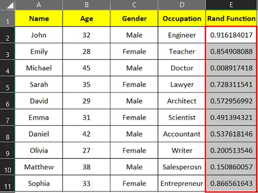
• Copy the formula down to assign random numbers to all rows. To do this, click on the bottom right corner of cell E2 and drag it down to the last row of your data.

Step 4 – Convert Formula Into Values

• Select the cells with the formula.
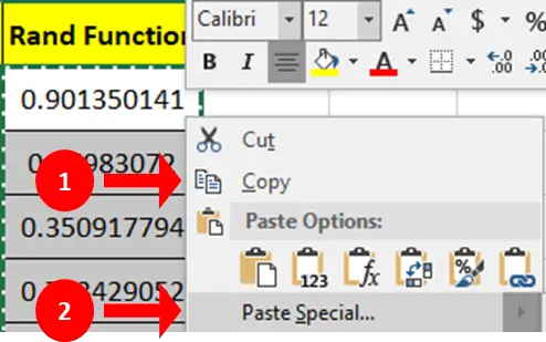
• Right-click on the selection, and choose “Copy” from the context menu.
• Again, right-click on the selected column, and choose “Paste Special” from the context menu.

Step 5 – Paste Special Dialog Box

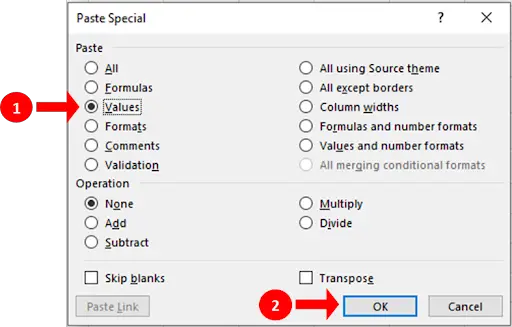
• In the “Paste Special” dialog box, select “Values” and click “OK.”
• Now, the formula will be converted into values. The purpose of this step is to have fix values instead of random while sorting the data.

Step 6 – Sort Data

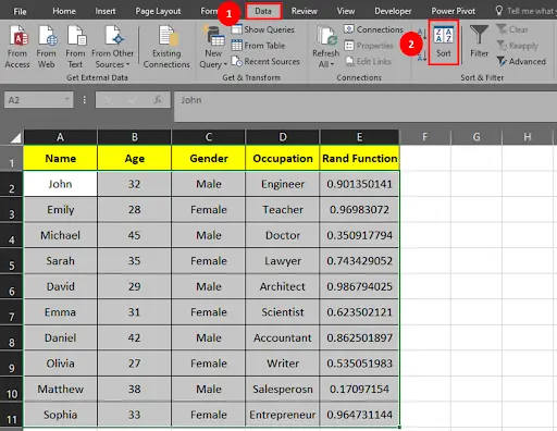
• Select the entire data range.
• On the Excel menu, go to the “Data” tab under Sort & Filter group, click on “Sort” button. A “Sort” dialog box will appear.

Step 7 – Sort Dialog Box

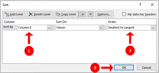
• In the “Sort by” drop-down menu, select the column that contains the random numbers (column E in this example).
• Choose “Smallest to Largest” in the “Order” drop-down menu.
• Click the OK button.
• Now, the rows in your data will be sorted based on the random numbers.

Step 8 – Rows Are Ready To Select Randomly

• You can now work with the randomly selected rows in Excel. If you need to select a specific number of random rows, you can simply take the top ‘n’ rows after sorting.

Method 2 – Use Of Index Function In Combination of RANDBETWEEN & ROWS Function

We will find a random name in this example.

Step 1 – Select The Cell 

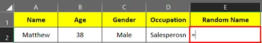
• Select the cell where you want to have random numbers, starting with equals (=) to sign.

Step 2 – Type The Formula

• In cell E2 type the formula.
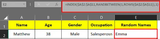
• =INDEX($A$2:$A$11,RANDBETWEEN(1,ROWS($A$2:$A$11)),1)
• Press the enter button.

Step 3 – Random Name Selected

• We can use this formula to find random names, numbers, etc.

Formula Breakdown:

We have used the following formula in this tutorial,

=INDEX($A$2:$A$11,RANDBETWEEN(1,ROWS($A$2:$A$11)),1)

The above formula is used to randomly select a value from a range of cells. Let’s break down the components of this formula.

• INDEX($A$2:$A$11: The INDEX function is used to retrieve a value from a specified range based on its position. In this case, the range being referenced is $A$2:$A$11, which represents the values in column A from row 2 to row 11.
• RANDBETWEEN(1,ROWS($A$2:$A$11)): The RANDBETWEEN function generates a random number between the two specified values. In this case, it generates a random number between 1 (the first row) and the total number of rows in the range $A$2:$A$11, which is obtained using the ROWS function. This ensures that the generated random number falls within the range of valid row numbers.
• By combining these functions, the formula selects a random row number within the range of $A$2:$A$11, and then uses the INDEX function to retrieve the value from column A at that randomly selected row.