
How to paste data Vertical in Excel
 By
SpreadCheaters
By
SpreadCheaters
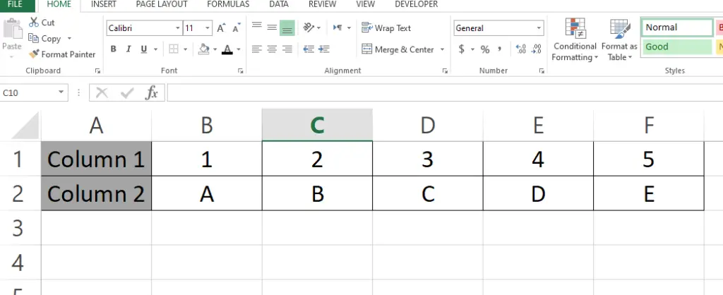
Here we have a simple dataset with two columns and 5 rows as an example. We will be copying the dataset and pasting it in a vertical position by following the steps below. Let’s have a look at the dataset first above.
Pasting vertically can also be useful when you need to reorganize data in a spreadsheet. For example, you might have a spreadsheet with a column of dates and a column of corresponding sales figures, and you want to reorganize the data so that the dates and sales figures are both in the same column.
Step 1 – Select the Data.
– Select the data you want to paste vertically.
– Copy the selected data by Ctrl + C.
– Select the cell where you want to paste the data.
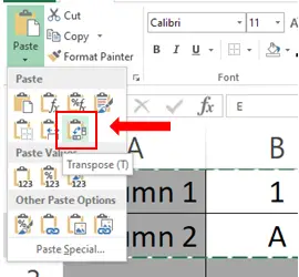
– In the Home tab open the dropdown menu for Paste.
– Choose Transpose from the Icon shown in the screenshot above.
Step 2 – Click on Transpose.

– After you click on the Transpose icon, copied data will be pasted to the selected cell vertically.
– Data will be pasted as shown above.


