
How to normalize data in Excel
 By
SpreadCheaters
By
SpreadCheaters
You can watch a video tutorial here.
Normalizing data is the process of scaling a set of data so that the values fall between 0 and 1. This is useful when comparing 2 sets of data that have different scales. This technique is widely used as part of data preprocessing in machine learning, to improve the performance of a statistical model. Excel does not have a built-in formula for normalization, but you can normalize data in Excel using regular mathematical formulas. The process is as follows:
- Find the minimum value of the dataset
- Find the maximum value of the dataset
- Compute the difference between the maximum and the minimum
- For each value in the dataset, subtract the minimum value and divide by the difference
In this example, we will use the sales value and the number of customers for each branch of a store to find out which branch has performed the best. As both sets of data have different scales (one is the number of people and the other is the currency value), the datasets have to be normalized before comparing them.
Step 1 – Find the minimum value of each dataset using MIN()
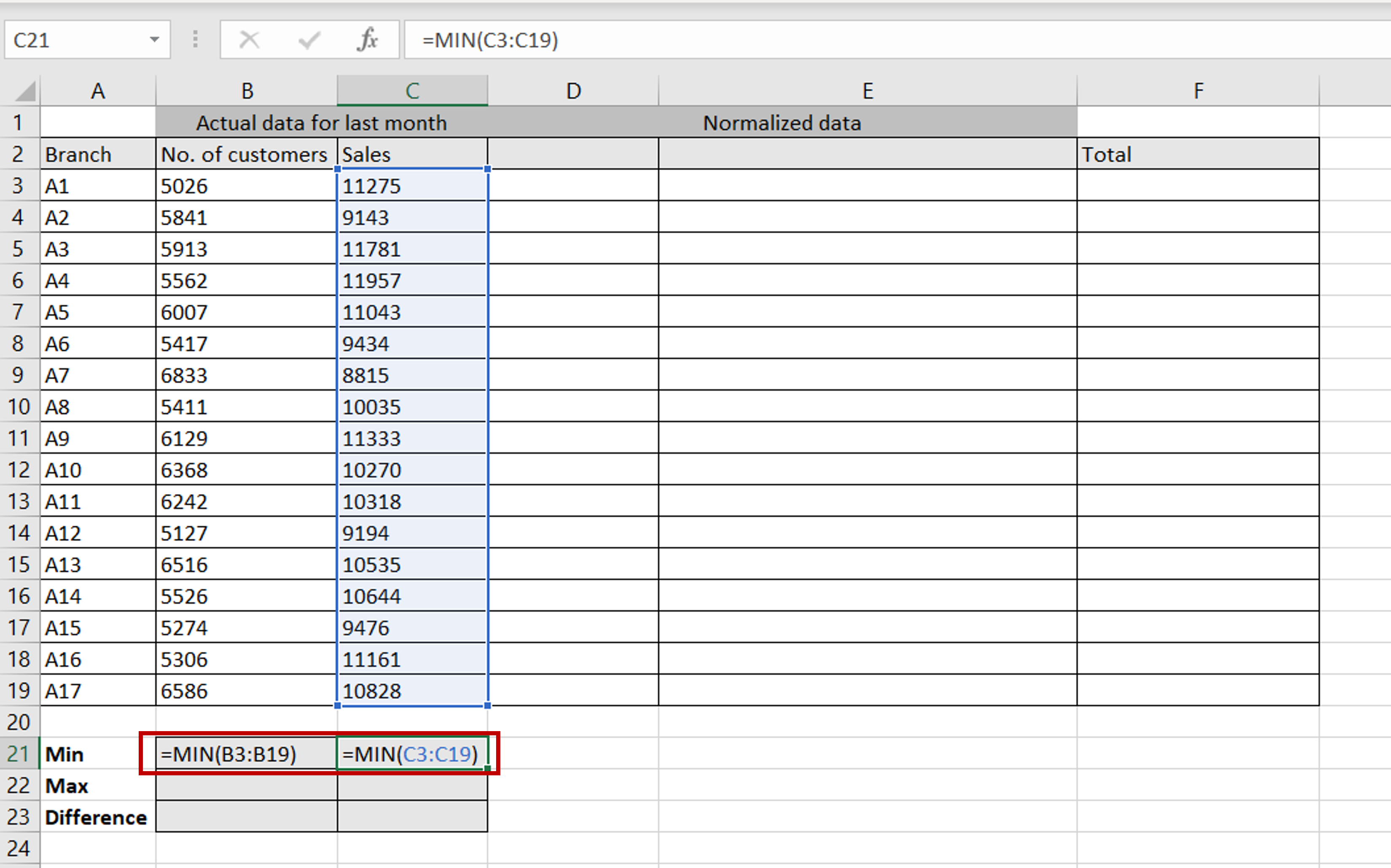
– In the destination cell, type the formula:
=min(<range of values>)
– Copy and paste the formula (Ctrl+C, Ctrl +V) to the next cell, for the next dataset
Step 2 – Find the maximum value of each dataset using MAX()
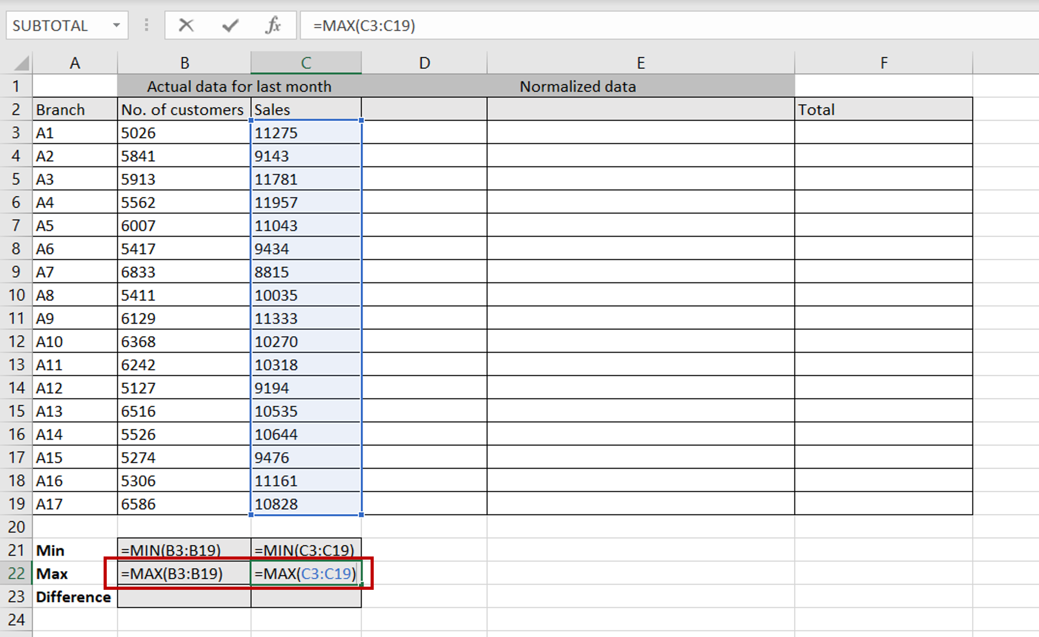
– In the destination cell, type the formula:
=max(<range of values>)
– Copy and paste the formula (Ctrl+C, Ctrl +V) to the next cell, for the next dataset
Step 3 – Find the difference between the maximum value and minimum value of each dataset
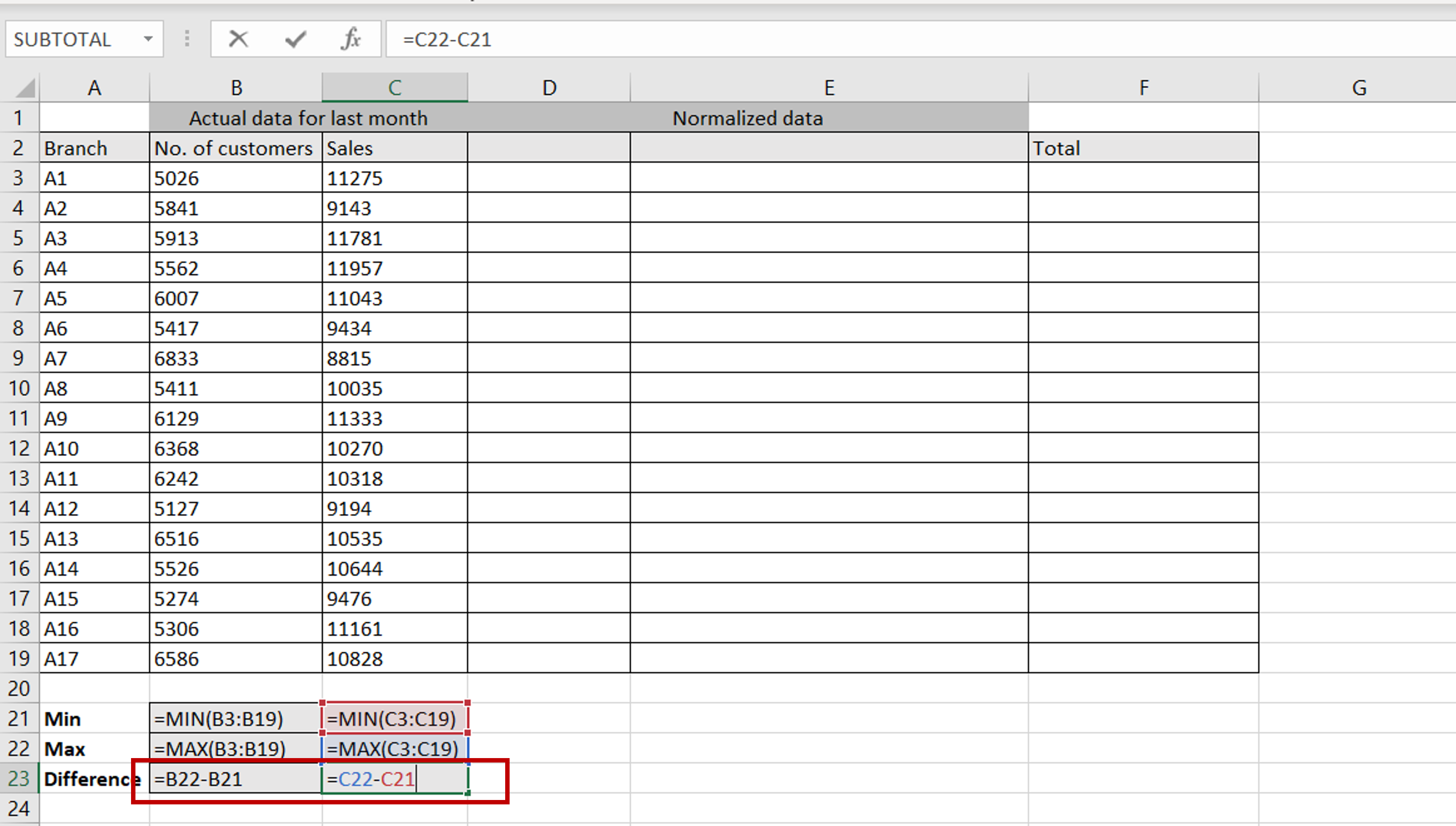
– In the destination cell, type the formula:
=<cell reference of the maximum value> – <cell reference of the minimum value> –
– Copy and paste the formula (Ctrl+C, Ctrl +V) to the next cell, for the next dataset
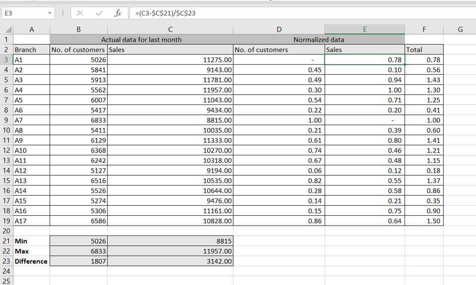
Step 4 – Enter the formula for normalizing data
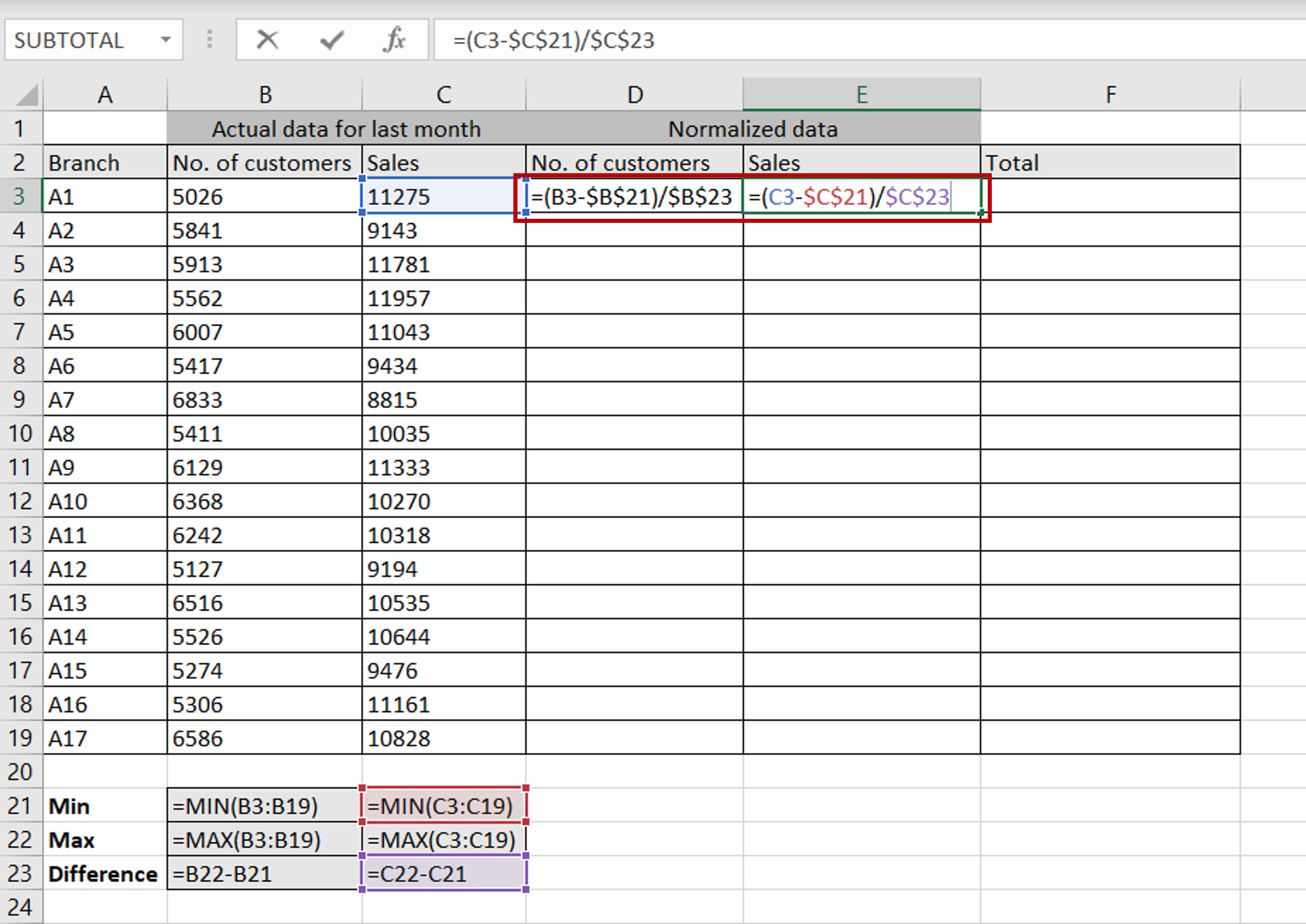
– In the first cell of the column that will contain the normalized values for the number of customers, type the formula for scaling:
= (<cell reference of the first value in the ‘No. of customers’ column> –
<minimum value of the ‘No. of customers’ dataset)/
<difference of the ‘No. of customers’ dataset
– Make the cell references for the minimum value and the difference constant by adding dollar signs ($)
– Enter the same formula in the first cell of the normalized ‘Sales’ column
Step 5 – Copy the formulas to the rest of the columns
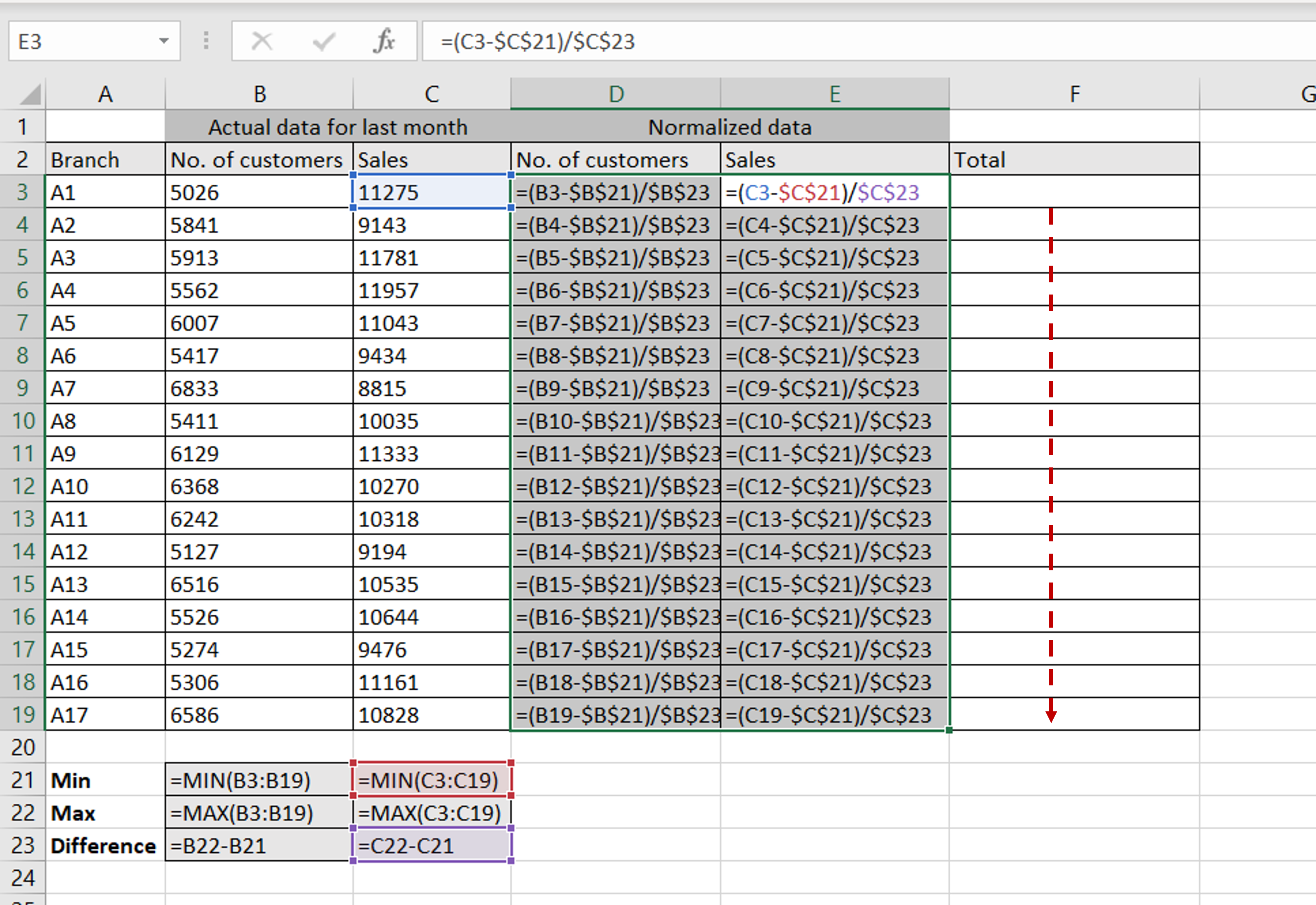
– Using the fill handle from the first cell, drag the formula to the remaining cells
OR
a) Select the cell with the formula and press Ctrl+C or choose Copy from the context menu (right-click)
b) Select the rest of the cells in the column and press Ctrl+V or choose Paste from the context menu (right-click)
Step 6 – Sum the normalized values
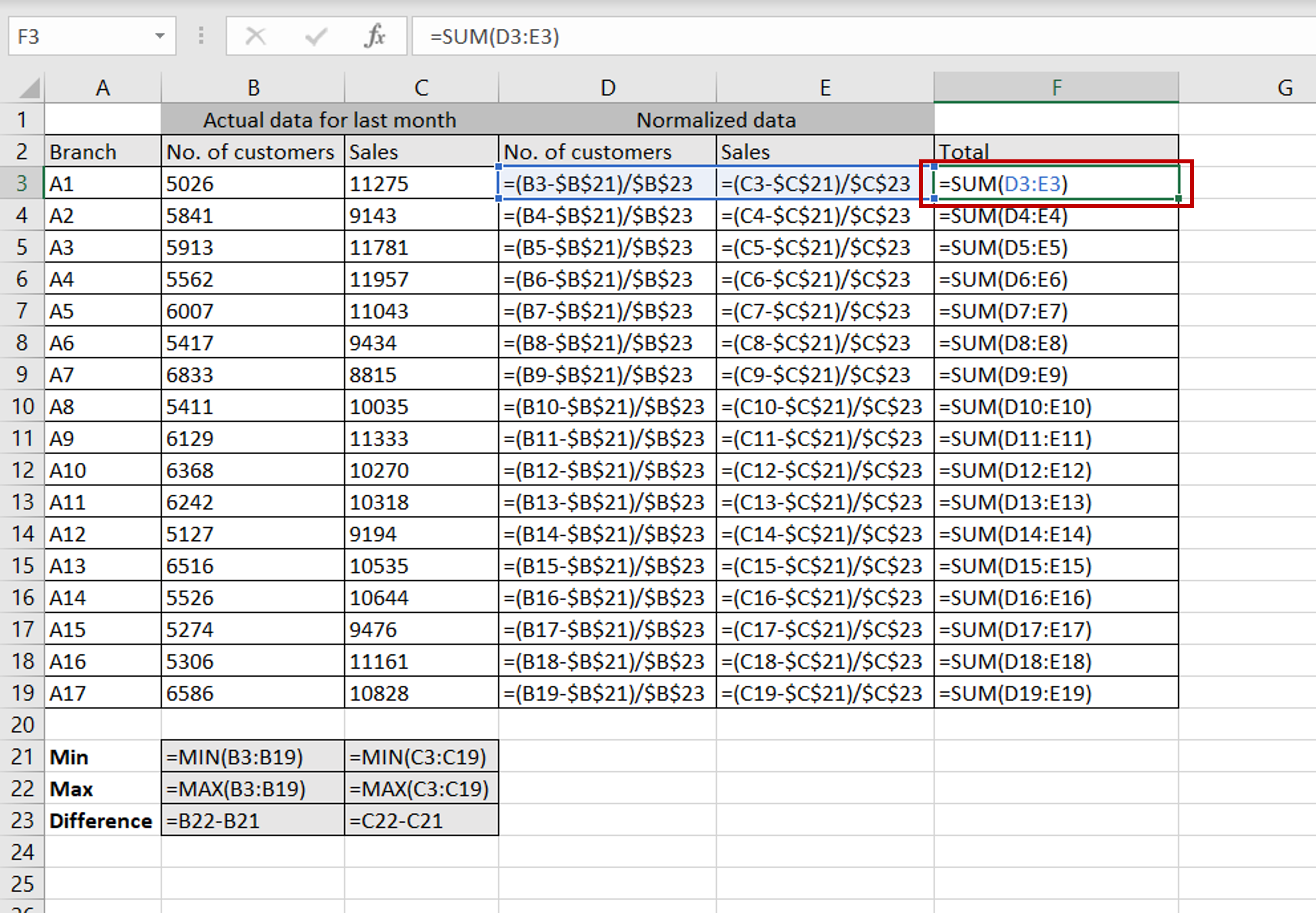
– For each branch, add the normalized ‘No. of people’ to the normalized ‘Sales’
Step 7 – Compare the data
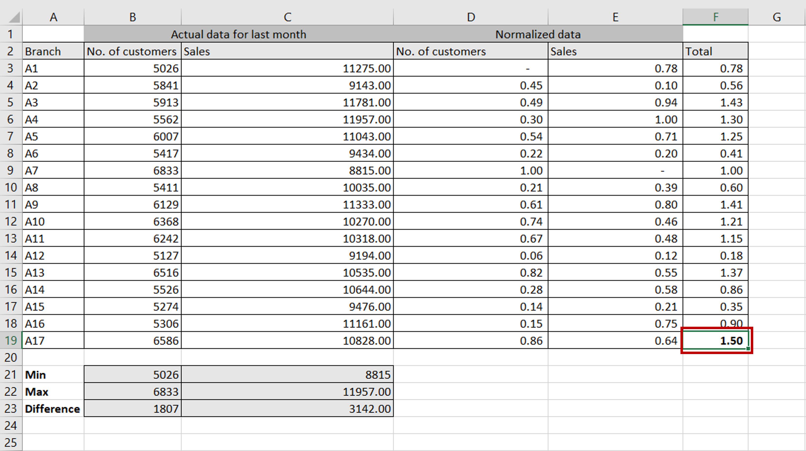
– Each dataset ranges from 0 to 1 with the minimum value being 0 and the maximum value being 1
– In comparison with all the other branches, branch A17 has performed the best


