How To Nest A Match Function In Excel

In this article, we will learn how to nest the MATCH function in Excel with an example and see how to use this technique to analyze our data more effectively.

First, let’s understand what the MATCH function does in Excel. The MATCH function searches for a specified value in an array and returns its position.

The syntax for the MATCH function is:

=MATCH(lookup_value, lookup_array, [match_type])

lookup_value: The value to search for.

lookup_array: The range of cells to search in.

match_type: An optional argument that specifies whether to find an exact match or an approximate match. If omitted, it defaults to 0 (exact match).

Now let’s move on to nest the MATCH function, which means using the result of one MATCH function as the lookup value for another function. Here’s an example of how to do it step by step.

Suppose we have a list of fruits and their prices in a table as shown below:

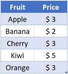
We want to find the position of a particular fruit in the list, but we don’t know the exact location of the fruit. We can use the MATCH function to find the position of the fruit and then use that position as the lookup value for another MATCH function to find its price.

Excel is a powerful tool for managing and analyzing data, but sometimes it can be challenging to extract the exact information you need from a large dataset. One way to make your data analysis more efficient is to use the MATCH function in Excel, which allows you to find the position of a particular value within a range of cells. However, you can also nest the MATCH function within other functions to create more complex formulas that can help you extract, analyze, and visualize your data in different ways.

Step 1 – Select The Cell

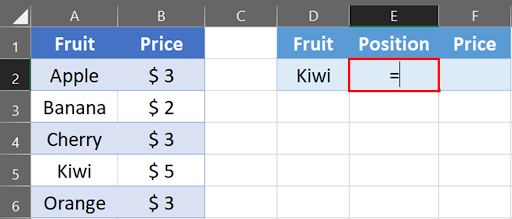
– Start by selecting the cell where you want to display the result of the MATCH function. Let’s say we want to display the position of “Kiwi” in cell E2.
– Place equals (=) to sign.

Step 2 – Type The Formula

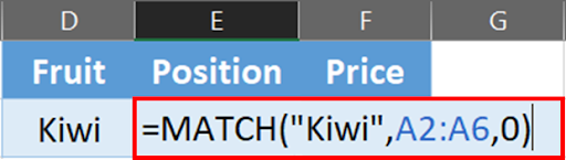
– Type the following formula: =MATCH(“Kiwi”, A2:A6, 0).

Step 3 – Press Enter

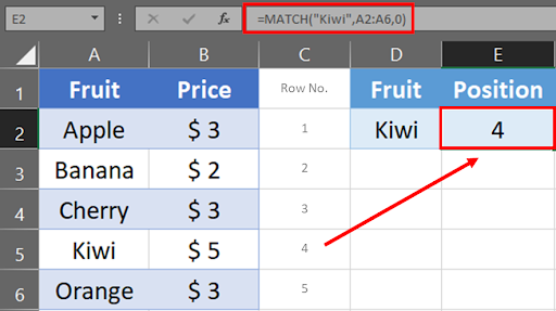
– Press Enter to see the result. In our example, the result is “4” because “Kiwi” is in the fourth row of the table.

Step 4 – Nest The MATCH Function With INDEX Function

– Now that we have the position of “Kiwi”, we can use it as the lookup value for another MATCH function to find its price.
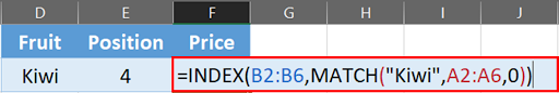
– Type the following formula in cell F2: =INDEX(B2:B6,MATCH(“Kiwi”,A2:A6,0))

Step 5 – Press Enter

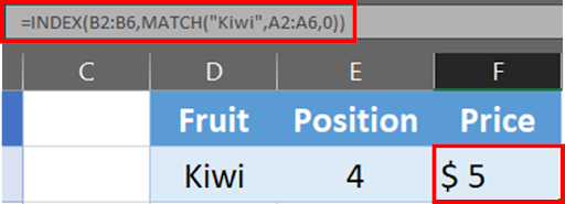
– Press Enter to see the result. In our example, the result is “$5” because the price of “Kiwi” is $5.

Step 6 – MATCH Function Nested

– This is how you can nest MATCH Function in Excel.

Formula Breakdown

=MATCH(“Kiwi”,A2:A6,0)

Here’s a breakdown of the formula:

• MATCH is a built-in function in Excel that searches for a specified value in a range of cells, and returns the position of the cell that contains the value.
• “Kiwi” is the value that we’re searching for in the range of cells A2 to A6. This could be any text, number, or logical value.
• A2:A6 is the range of cells that we’re searching in. In this case, we’re searching for the value “Kiwi” in the cells A2, A3, A4, A5, and A6.
• 0 is the match type. This indicates that we’re looking for an exact match. If the value “Kiwi” is not found in the range of cells A2 to A6, the formula will return the #N/A error.

So, when we put it all together, the formula =MATCH(“Kiwi”,A2:A6,0) searches for the value “Kiwi” in the range of cells A2 to A6, and returns the position of the first cell in the range that contains the value “Kiwi”. If “Kiwi” is not found, the formula returns the #N/A error.

=INDEX(B2:B6,MATCH(“Kiwi”,A2:A6,0))

Here’s a breakdown of the formula:

• INDEX is a built-in function in Excel that returns a value or reference to a cell at the intersection of a particular row and column in a range.
• B2:B6 is the range of cells that we want to return a value from. In this case, we want to return a value from the cells B2, B3, B4, B5, and B6.
• MATCH(“Kiwi”,A2:A6,0) is a nested formula that returns the position of the first cell in the range of cells A2 to A6 that contains the value “Kiwi”, using the same logic as the formula above. This position is then used as the row number in the INDEX function.

So, when we put it all together, the formula =INDEX(B2:B6,MATCH(“Kiwi”,A2:A6,0)) returns the value from the cell in the range B2 to B6 that corresponds to the position of the first cell in the range A2 to A6 that contains the value “Kiwi”. If “Kiwi” is not found in the range A2 to A6, the formula returns the #N/A error.