How to merge duplicates in Excel

You can watch a video tutorial here.

Excel is a spreadsheet application which lends itself easily to creating lists, tables, and databases. When combining data from multiple sources, you will frequently encounter rows that have duplicate values. To analyze the data or to prepare a summary, you will need to merge the duplicates. When merging the duplicates, you also need to specify how the values associated with the duplicates will be aggregated (e.g. sum, count). In Excel, there are 2 ways of doing this. 

Option 1 – Create a pivot table

Step 1 – Select the data

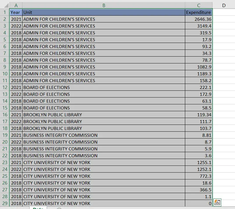
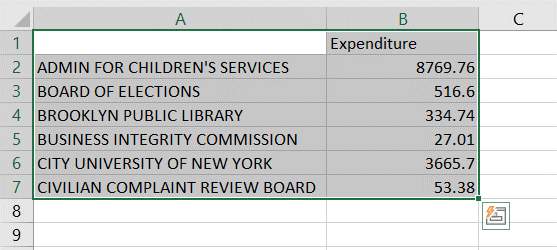
• Select all the data that contains duplicates

Step 2 – Open the PivotTable from table or range box

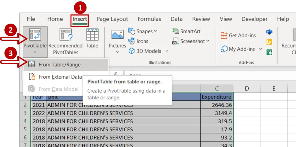
• Go to Insert > Tables
• Expand the PivotTable dropdown
• Select From Table/Range

Step 3 – Check the settings

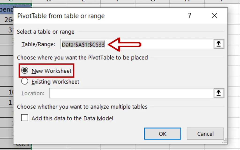
• The range is automatically populated
• Choose New Worksheet
• Click OK

Step 4 – Define the Pivot table structure

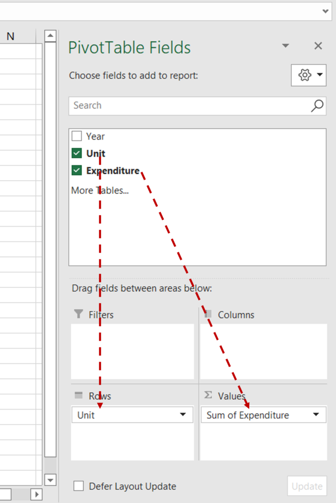
• Drag ‘Unit’ into the the Rows pane
• Drag ‘Expenditure’ into the Values pane
• The ‘Expenditure’ is automatically summed

Step 5 – Check the result

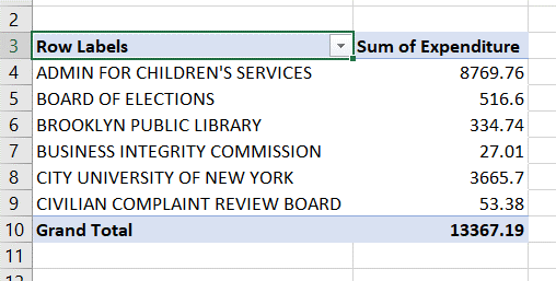
• The Pivot table is created
• The rows containing duplicates of ‘Unit’ are merged and the ‘Expenditure’ values are summed

Option 2 – Consolidate the data

Step 1 – Select the destination

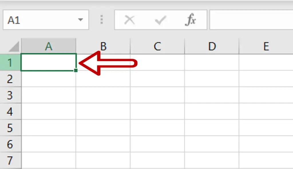
• Select the cell from which the merged data is to be placed

Step 2 – Open the Consolidate box

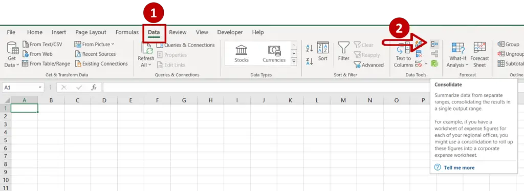
• Go to Data > Data Tools
• Click on the Consolidate button

Step 3 – Select the data

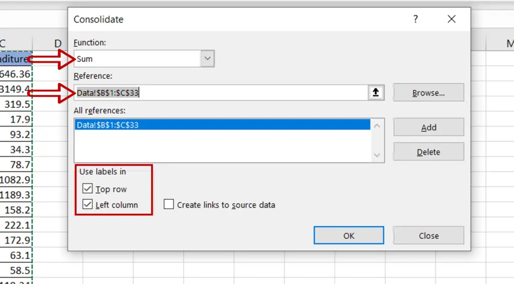
• Choose the Sum  function
• Place the cursor in the Reference box
• Select the ‘Unit’ and ‘Expenditure’ columns
• Click Add
• Tick Use labels in:
  • Top row
  • Left column
• Click OK

Step 4 – Check the result

• The data in both sheets are merged into a single table
• The expenditure for the rows that have the same ‘Unit’ is added