How To Merge Cells Vertically In Excel

Excel is not just a basic spreadsheet program; it’s a powerful tool that empowers users to manipulate data and present it in a meaningful way. One technique that can significantly enhance the visual appeal and readability of your Excel worksheets is merging cells vertically. By merging cells, you can seamlessly combine information from multiple cells into a single cell, creating a more structured and concise representation of your data. 

Join us in this step by step guide, as we uncover the methods to vertically merge cells in Excel, and witness how this simple yet impactful feature can elevate your data presentation skills.

Method 1 – Using CONCATENATE Function

The CONCATENATE function in Excel is a text function that allows you to combine (concatenate) multiple strings of text into a single string. It helps you create new text values by joining together existing text values, cell references, or a combination of both. The CONCATENATE function is particularly useful when you need to merge data from different cells or add additional text or characters between them.

Formula Syntax 

The general syntax of the CONCATENATE function is as follows:

=CONCATENATE(text1, [text2], [text3], …)

Here’s a breakdown of the function’s components:

• text1, text2, text3, and so on: These are the text values or cell references that you want to concatenate. You can specify up to 255 arguments. Each argument can be a text string enclosed in quotation marks (e.g., “Hello”) or a cell reference (e.g., A1).
• [text2], [text3], and so on: These are optional arguments. You can include as many or as few as needed. If an argument is omitted, it won’t affect the concatenation.

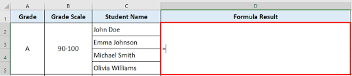
Step 1 – Select The Cell

• Select the cell where you want to enter the formula & place equals (=) to sign.

Step 2 – Type The Formula

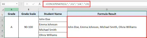
• Now start typing the formula in cell D2.

=CONCATENATE(C2,”, “,C3,”, “,C4,”, “,C5). This formula will take all text vertically from the cells C2, C3, C4 and C5 from Column C, and then merge them with a space in between.

• Now press enter to apply the formula and get the desired results as above.

Step 3 – Text Merged In The Cell

• All the text merged in a single cell without losing formatting & data as shown in the image.

Method 2 – Using Ampersand Symbol

To join the text from a group of cells, we can also use the Ampersand symbol. The operator joins the text into a single cell.

Step 1 – Select The Cell

• Select the cell where you want to enter the formula & place equals (=) to sign.

Step 2 – Type The Formula

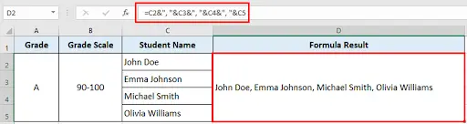
• Now start typing the formula in cell D2.

=C2&”, “&C3&”, “&C4&”, “&C5

• This simple formula uses ampersand operator and merge vertically the cells of the Column C with a space after each cell. Now press enter to apply the formula.

Step 3 – Text Merged In The Cell

• All the text merged in a single cell without losing formatting & data.

Method 3 – Using CONCAT Function

The CONCAT function combines the text from multiple ranges and/or strings, but it doesn’t provide delimiter or ignore empty arguments. 

CONCAT replaces the CONCATENATE function. However, the CONCATENATE function will stay available for compatibility with earlier versions of Excel.

Formula Syntax

=CONCAT(text1, [text2],…)

Here’s a breakdown of the function’s components:

• text1 (required): Text item to be joined. A string, or array of strings, such as a range of cells.
• [text2, …] (optional): Additional text items to be joined. There can be a maximum of 253 text arguments for the text items. Each can be a string, or array of strings, such as a range of cells.

We will be using the following dataset for this method. Also, we will be using two techniques to apply the formula.

The difference between the two techniques is the space after every word in the text column.

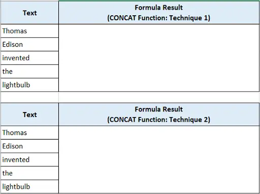
Technique 1 Using CONCAT with a Range of Cells

Step 1 – Select The Cell

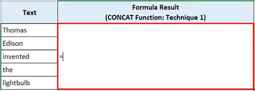
• Select the cell where you want to insert the formula & place equals to (=) sign.

Step 2 – Type The Formula

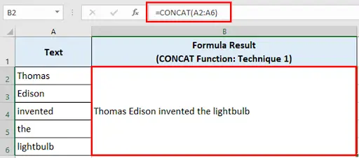
• Typing the formula in cell B2.
• =CONCAT(A2:A6)
• The above formula will combine the range mentioned inside and merge it in one cell where the formula is applied. To apply the formula press enter and get desired results.

Step 3 – Text Merged

• All the text will be merged in a single cell.

Technique 2 Using CONCAT with individual cells

Step 1 – Select The Cell

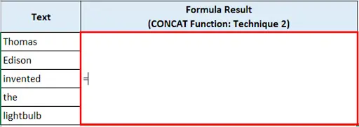
• Select the cell where you want to insert the formula & place equals to (=) sign.

Step 2 – Type The Formula

• Typing the formula in cell B2.
• =CONCAT(A9,” “,A10,” “,A11,” “,A12,” “,A13)
• Press enter to apply the formula.

Step 3 – Text Merged

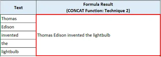
• All the text will be merged in a single cell.

Method 4 – TEXTJOIN Function

The TEXTJOIN function combines the text from multiple ranges and/or strings, and includes a delimiter you specify between each text value that will be combined. If the delimiter is an empty text string, this function will effectively concatenate the ranges. Personally, I prefer this method over all other methods because it gives the liberty to choose and mention the delimiter only once in the formula and all text will be embedded with that delimiter.

Syntax

=TEXTJOIN(delimiter, ignore_empty, text1, [text2], …)

• delimiter (required): A text string, either empty, or one or more characters enclosed by double quotes, or a reference to a valid text string. If a number is supplied, it will be treated as text.
• ignore_empty (required): If TRUE, ignores empty cells.
• text1 (required): Text item to be joined. A text string, or array of strings, such as a range of cells.
• [text2, …] (optional): Additional text items to be joined. There can be a maximum of 252 text arguments for the text items, including text1. Each can be a text string, or array of strings, such as a range of cells.

This function can be used with individual cells and over the range as well, for example

Step 1 – Select The Cell

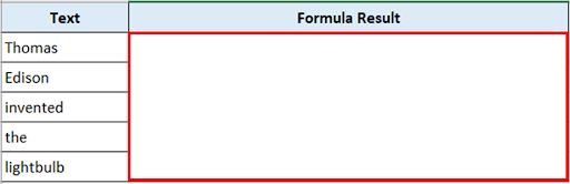
• Select the cell where you want to insert the formula & place equals to (=) sign.

Step 2 – Type The Formula

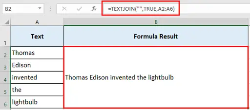
• Typing the formula in cell B2.
• =TEXTJOIN(“”,TRUE,A2:A6)
• Press enter to apply the formula.

Step 3 – Text Merged

• All the text will be merged in a single cell.