How to match one column to another in Excel

Excel column matching is something that we all occasionally do. There are several choices for matching data in Microsoft Excel, but the majority of them concentrate on searching in a single column. In this article, we’ll look at a variety of methods for matching two columns in Excel and identifying similarities and differences.

Method 1 – Using Formula IF CONDITION

The syntax of the IF function is as follows;

=IF(Logical_test,value_IF_true,value_IF_false)

Arguments:

The condition we wish to examine is logical_test. When comparing the numbers in cells A2 and B2, our situation is A2=B2.

The value or expression that must be returned if the logical_test is true is designated as value_if_true. It will be “Match” in our situation.

If the logical_test is false, value_if_false is the value or expression that ought to be returned. It will return “NO MATCH” in our situation.

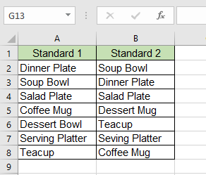
Suppose below is the data set

Step – 1 – Add a new column

• Add the column in the data set.
• Give the name to added column as match / no match, see the below image.

Step – 2 – Apply Formula

• Write the following formula in column C

=IF(A2=B2,”Match”,”NO MATCH”)

• Press “Enter”

Step – 3 – Drag the Formula

• Now drag the formula downwards to find out matching

Method 2 – Using Formula IF AND Condition

An IF formula with an AND statement will work great if your table has three or more columns and you want to locate rows that have identical values in all cells.

Step – 1 – Apply Formula

• Write down to following formula in column D

=IF(AND(A2=B2, A2=C2), “Perfect match”, “Not Match”)

• Press “Enter”.

Step – 2 – Drag the Formula

• Drag the formula downwards to apply it on all rows.

Method 3 – Using IF & EXACT Function

Use the EXACT function to identify case-sensitive matches between two columns in each row. Enter the corresponding text (“Different” in this example) in the third argument of the IF function to identify case-sensitive differences in the same row.

Step – 1 – Apply Formula

• Write the following formula in Column C

=IF(EXACT(A2, B2), “Match”, “Different”)

• Press “Enter”

Step – 2 – Drag the Formula

• Drag the formula downwards for the application

Method 4 – Using Conditional Formatting

Step – 1 – Apply Conditional Formatting

• Select the data
• Click on the conditional Formatting option on the home tab in the styles group.
• A drop down menu will appear.
• Choose the highlight cell rules option.
• Another side menu will open and choose Duplicate Values from this menu.
• Click on the “OK” button. This will implement the conditional formatting on the data and the matching entries in both columns will be highlighted.