
How to manually sort Data in pivot table in Excel
 By
SpreadCheaters
By
SpreadCheaters
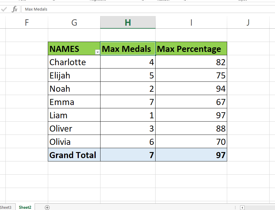
In this tutorial, we’ll show you how to manually sort data in a pivot table. Here we have a dataset which contains 3 columns, First column contains NAMES, Second column contains MAX Medals achieved by the students and last column contains their MAX Percentage. We will be re-arranging some rows and columns in this pivot table manually. Steps to do it are given below but first we will have a look at the dataset above.

Pivot tables are a powerful tool for analyzing and summarizing large amounts of data in Microsoft Excel. By default, pivot tables are sorted in alphabetical or numerical order based on the values in the rows and columns. However, sometimes you may want to sort the data in a different way to better understand the trends and patterns in your data.
Step 1 – Rearrange the Row
– To rearrange the row select the cell of the row.
– Move the cursor to the border of the cell.
– When a 4 arrow shaped cursor appears, click and drag the row to the desired location.
– In our case we have moved Emma to the top.
Step 2 – Rearrange the column

– To rearrange the column select the cell of the column.
– Move the cursor to the border of the cell.
– When a 4 arrow shaped cursor appears, click and drag the column to the desired location.
– In our case we moved MAX Percentage to the place of the second column.


