
How to make subcategories in Microsoft Excel
 By
SpreadCheaters
By
SpreadCheaters
In this tutorial, we will learn how to make subcategories in Microsoft Excel. In Excel making subcategories is a useful task. It is mostly accomplished by utilizing the Data Validation feature and Named Ranges.
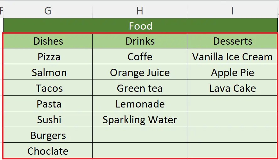
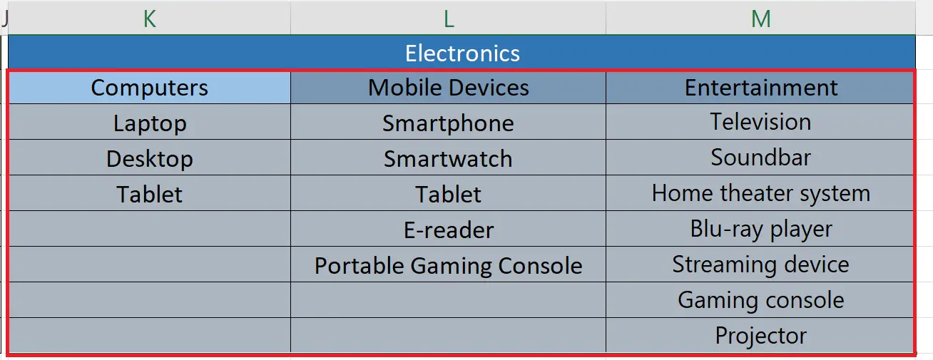
Currently, we possess data representing two primary categories: Food and Electronics. Furthermore, within each category, there are three subcategories. Our objective is to employ Data Validation and Named Ranges to generate these subcategories.

Creating subcategories in Excel involves establishing a relationship between cells, where the options available in one cell depend on the selection made in another cell. This technique allows for dynamic updates and helps ensure data accuracy and a streamlined data entry process. These subcategories may also be named dependent lists.
Step 1 – Organize the Data in Proper Rows and Columns
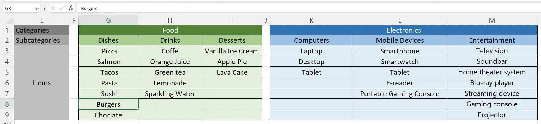
– Organize the data by placing the appropriate headers in each row. This involves setting headers for each category and, under each category, setting headers for the subcategories.
– List the items for each subcategory under the headers.
Step 2 – List the Primary Categories Separately
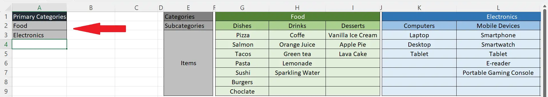
– List the primary categories separately aside from the original data set.
Step 3 – List the Subcategries for Each
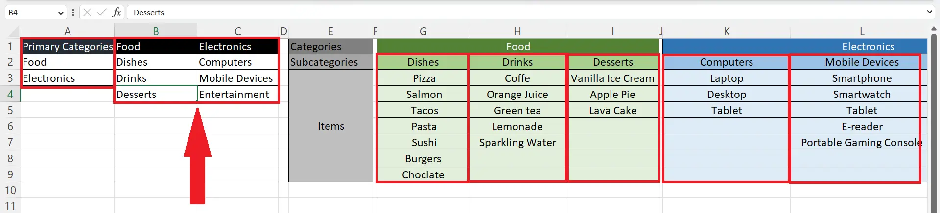
– List the headers of subcategories for each separately under the header of the primary category.
– Now we, have separate columns for each list i.e. a list of headers of primary categories, a list of subcategories, and a list of items for each subcategory in the original data set.
Step 4 – Create a Named Range for the Primary Category “Food”
– Create a named range for the primary category “Food”.
– Select the columns in which you have listed all the subcategories for the primary category “Food”.
– Locate the “Create from Selection” button in the Formulas tab.
– Select the “Top row” option in the dialog box and hit the OK button.
Step 5 – Create a Named Range for the Primary Category “Electronics”
– Create a named range for the primary category “Electronics”.
– Select the columns in which you have listed all the subcategories for the primary category “Electronics”.
– Locate the “Create from Selection” button in the Formulas tab.
– Select the “Top row” option in the dialog box and hit the OK button.
Step 6 – Select the all the Food Items Listed under Respective Subcategory Header
– Select all the items, organized under the respective subcategory header for the primary category “Food”.
Step 7 – Create the Named Range for Each Subcategory
– Keeping all the items selected, locate the “Create from Selection” button in the Formulas tab.
– Select the “Top row” option and hit the OK button.
– A named range for each subcategory of Food will be created containing the respective items for each.
Step 8 – Select the all the Electronics Items Listed under Respective Subcategory Header
– Select all the items, organized under the respective subcategory header for the primary category “Electronics”.
Step 9 – Create the Named Range for Each Subcategory
– Keeping all the items selected, locate the “Create from Selection” button in the Formulas tab.
– Select the “Top row” option and hit the OK button.
– A named range for each subcategory of Electronics will be created containing the respective items for each.
Step 10 – Check the created named ranges
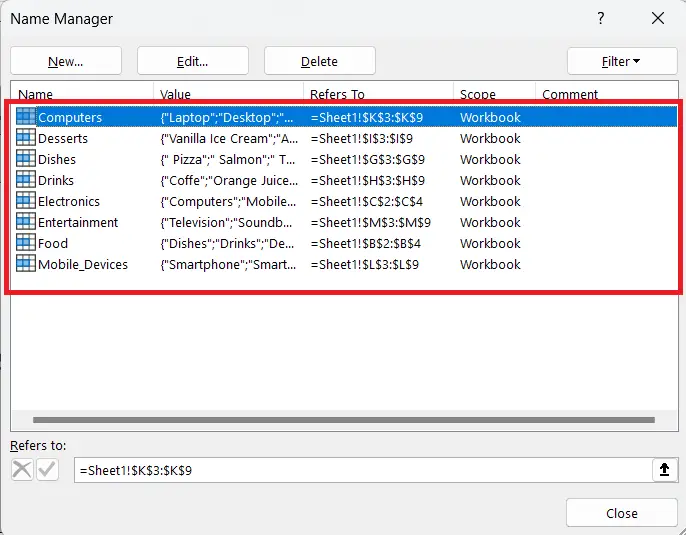
– The following 8 named ranges would be created. We can view them by clicking on the “Name Manager” button in the “Defined Names” section.
– Two named ranges of subcategories with the categories header i.e. Subcategories of Food and Electronics.
– Three named ranges of Food items under the headers of respective subcategories.
– Three named ranges of Electronics items under the headers of respective subcategories.
Step 11 – Choose the cells to create drop down lists
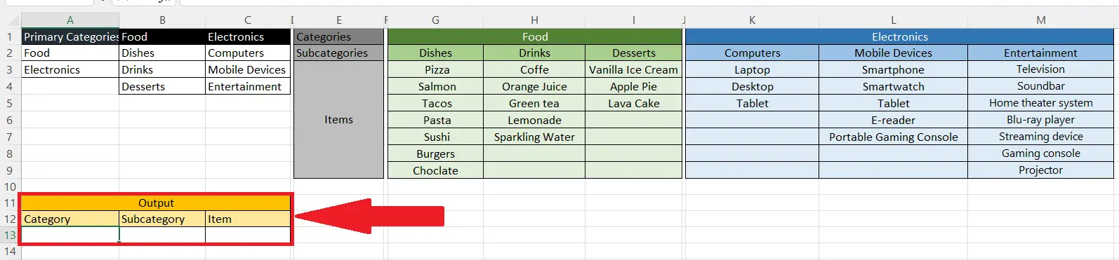
– Choose the destination where the final result is to be placed as drop down lists.
– Create the Following headers, each in a separate column: Category, Subcategory, and Items.
Step 12 – Choose the First Cell under the Category
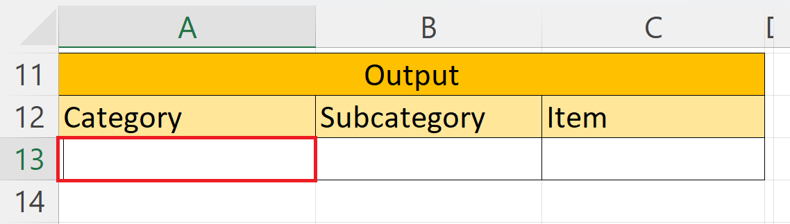
– Choose the first cell under the category header.
Step 13 – Create a List utilizing the Data validation Feature
– Create a list utilizing the “Data Validation” feature.
– Locate the Data Validation feature in the Data Tools section of the Data tab.
– Choose the list in the “Allow” drop-down menu.
– Enter the range containing the list of primary categories in the “Source” field. Do not include the header i.e. Primary Categories.
– Hit the OK button.
Step 14 – Choose the First Cell under the Subcategory
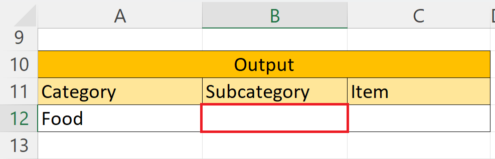
– Choose the first cell under the subcategory header.
Step 15 – Create a List utilizing the Data Validation Feature
– Create a list utilizing the Data Validation feature.
– Locate the Data Validation feature in the Data Tools section of the Data tab.
– Choose the list in the “Allow” drop-down menu.
– In the Source field, utilize the INDIRECT function and write =INDIRECT(A12).
– Where A12 is the cell reference of the first cell under the “Category” header as shown in the image.
Step 16 – Choose the First Cell under the Items
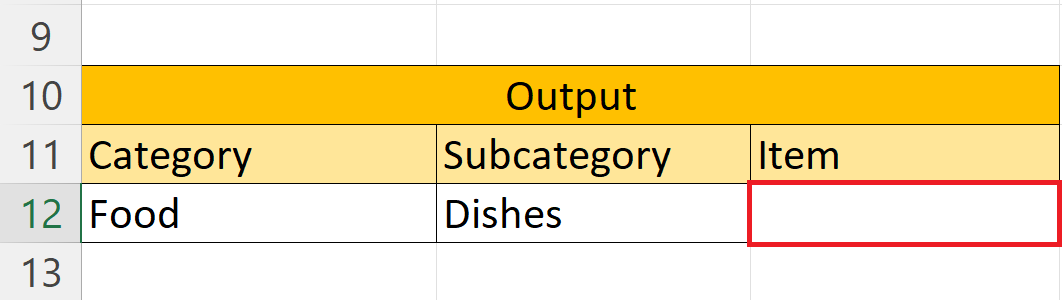
– Choose the first cell under the “Items” header.
Step 17 – Create a List utilizing the Data Validation Feature
– Create a list utilizing the Data Validation feature.
– Locate the Data Validation feature in the Data Tools section of the Data tab.
– Choose the list in the “Allow” drop-down menu.
– In the Source field, utilize the INDIRECT function and write =INDIRECT(B12).
– Where B12 is the cell reference of the first cell under the “Category” header as shown in the image.
Step 18 – Now Check the Final Output
– Now check the final output by selecting the primary category from the first column, the subcategory, and then an item under the subcategory.


