How to make Positive numbers negative in Excel

To make positive numbers negative in Excel means to convert all positive numbers in a given range or column to their negative equivalent. This can be useful for a variety of reasons, such as when you want to highlight losses or negative values in your data, or when you need to perform calculations that require negative numbers.

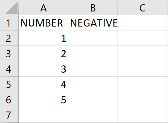
In this tutorial, we will learn how to make positive numbers negative in excel. Our dataset contains positive numbers, and we need to convert them to negative values. To do this, we have two methods available: the Paste Special function and the ABS function. Below are the steps to use these methods.

Method 1: Make all Numbers Negative in Different Cells

The ABS function in Excel is a built-in mathematical function that returns the absolute value of a number. The absolute value of a number is its magnitude without regard to its sign. The syntax of the ABS function is as follows:

=ABS(number)

The argument “number” is the value whose absolute value we want to find. This argument can be a cell reference that contains a numerical value or a numerical value directly entered into the function. The ABS function will return a positive value, regardless of whether the original value was positive or negative.

Step 1 – Select the Cell

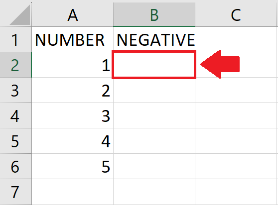
• Click on the cell, where you want to show the negative value

Step 2 – Use the ABS function with negative sign

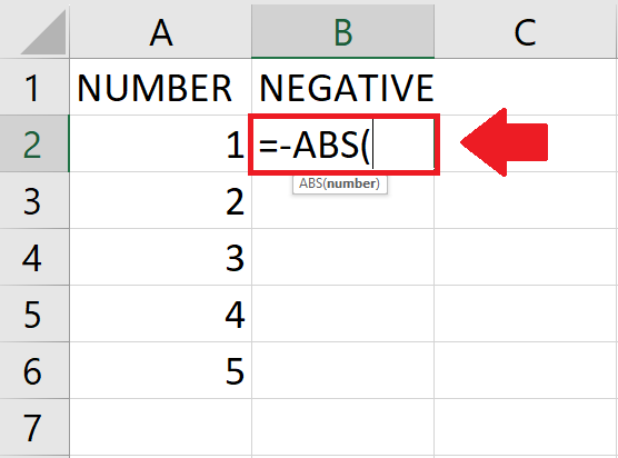
• To use Abs function type “ = – ABS( ” 

Step 3 – Type the Argument

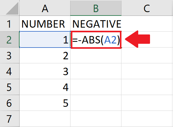
• Type the argument of the function
• Here the argument is the number
• We have used A2 as a number argument
• After typing the argument, type the closing bracket “ ) ”

Step 4 – Press Enter key

• After typing the argument, press Enter key to get the required result

Step 5 – Apply on the Entire Column

• To apply this action on the complete column, use autofill 

Method 2: Make All Numbers Negative in their cells

Step 1 – Type Negative 1 

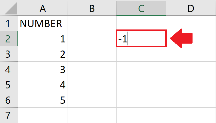
• Type “ -1 ” in any cell of the sheet

Step 2 – Copy the cell

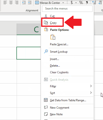
• After typing the negative one in the cell, copy it 
• To copy it open the context menu(by right-clicking on the cell) 
• In the context menu click on Copy option

Step 3 – Select the Range of Cells

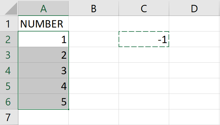
• After copying the cell, select the range of cells that you want to be negative

Step 4 – Click on the Paste special option in the Context menu

• After selecting the range of cells, Right click on the selected  range to open the context menu
• From the context menu, click on the Paste Special option and a dialog box will appear

Step 5 – Select the Multiply option

• In the dialog box, click on Multiply from the list above the operation option
• Click on Ok at the end of the dialog box to get the required result