How To Make Negative Numbers Red In Excel 2013

Are you tired of trying to find negative numbers in your Excel spreadsheets? One solution is to format them in red, making them easy to spot at a glance. In this tutorial, we will show you how to format negative numbers in red in Excel 2013, so you can work with your data more efficiently.

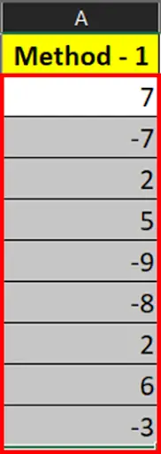
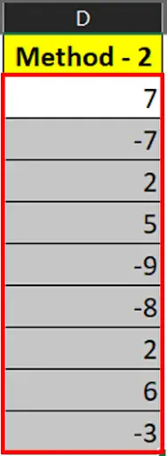
Suppose we have the data with both positive and negative numbers, and we only want to make the negative numbers red. You can do this by following the methods below.

Method 1 – Builtin Number Formatting

Step 1 – Select Data

• Select your data.

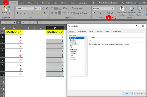
Step 2 – Go To The Home Tab

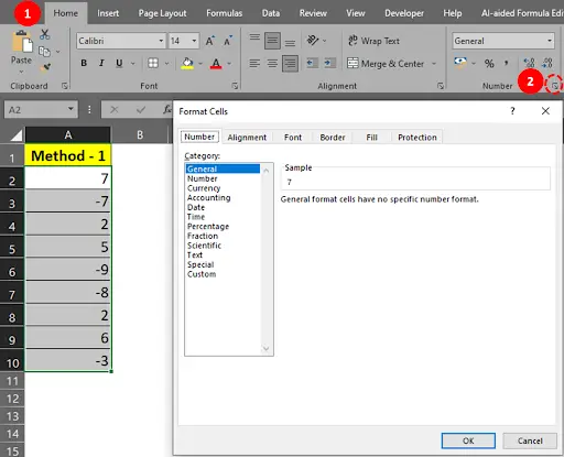
• Go to the Home Tab, under the Number group, click on the Number Format button.
• The Format Cells dialog box will appear on your screen.

Step 3 – Select Number Formatting

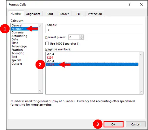
• In the Format Cells dialog box, under the Number tab, choose the Number category and select the negative number format of your choice.
• Click the OK button.

Step 4 – Negative Numbers Marked Red

• All the negative numbers in your data will be marked red.

Method 2 – Custom Number Formatting

Step 1 – Select Data

• Select your data.

Step 2 – Go To The Home Tab

• Go to the Home Tab, under the Number group, click on the Number Format button.
• The Format Cells dialog box will appear on your screen.

Step 3 – Set Custom Number Formatting

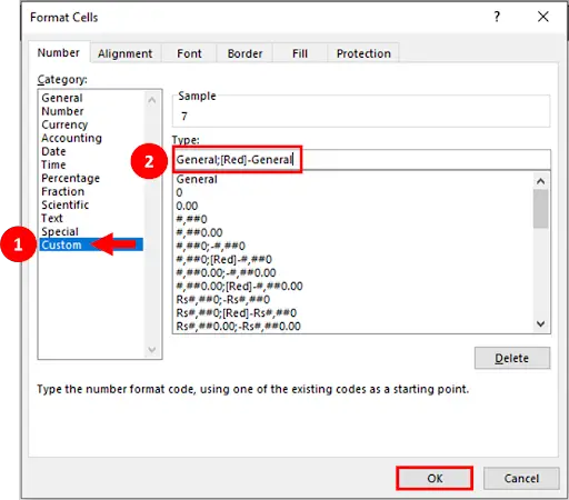
• In the Format Cells dialog box, under the Number tab, choose the Custom category.
• In the Type field, write a custom number format, i.e., “General;[Red]-General”.
• Click the OK button.

Step 4 – Number Marked Red

• All the negative numbers will be marked red.

Method 3 – Using Conditional Formatting

Step 1 – Select Data

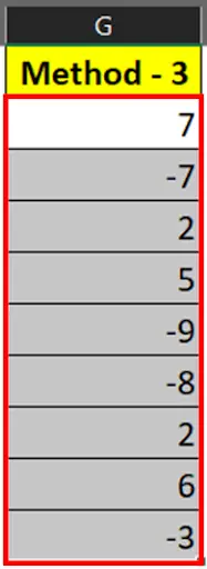
• Select your data.

Step 2 – Go To The Home Tab

• Go to the Home Tab, under the Styles group, click on the Conditional Formatting dropdown button.
• Hover your mouse over Highlight Cell Rules and select the Less Than option.

Step 3 – Set Condition

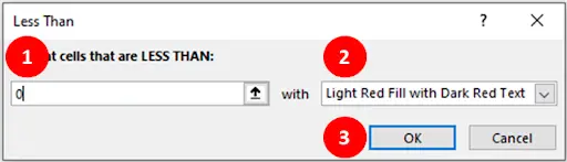
• A conditional formatting dialog box will appear on your screen.
• Type 0 (ZERO) as a less than condition. Change cell formatting if required. We will go with the default cell formatting and click the OK button.

Step 4 – Negative Numbers Highlighted In Red

• By applying conditional formatting, you can highlight cells having negative values as red.