
How To Make Negative Numbers Red In Excel
 By
SpreadCheaters
By
SpreadCheaters
Page last updated:
08/10/2022 |
Next review date:
08/10/2024
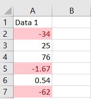
Formatting can be very handy when analyzing data. For this article, we’ll be focusing on conditional formatting and how to highlight negative numbers in Excel.
Step 1 – Highlight the cells
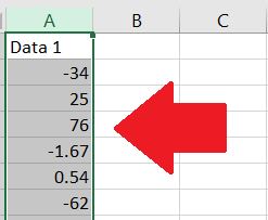
Highlight the cells that you want to format.
Step 2 – Under the Home tab, click on Conditional Formatting
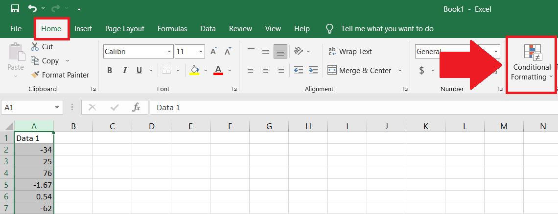
What conditional formatting does is change the color of the cell depending on a criteria.
Step 3 – Click on Highlight Cells Rules and Less Than
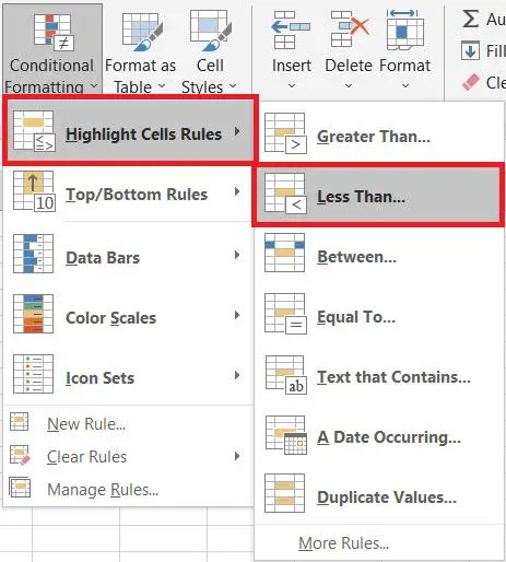
We click on Less Than since we want all negative numbers to be turned red.
Step 4 – A Format cells that are LESS than box will pop up. Add in 0 at the 1st box.
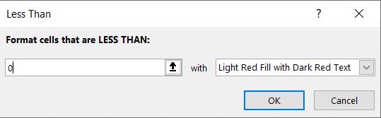
A Format cells that are LESS than box will pop up. Add in 0 at the 1st box.
Step 5 – Click OK.
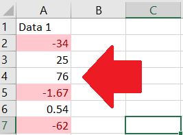
By clicking OK, all the selected cells will be highlighted in accordance with the criteria.


