How To Make Excel Count 1 2 3

Whether you’re a seasoned Excel user or just starting out, you may be wondering how to simply count from 1 to a specific number of cells. In this article, we’ll show you step-by-step how to make Excel count. There are many ways to do this, so let’s get started.

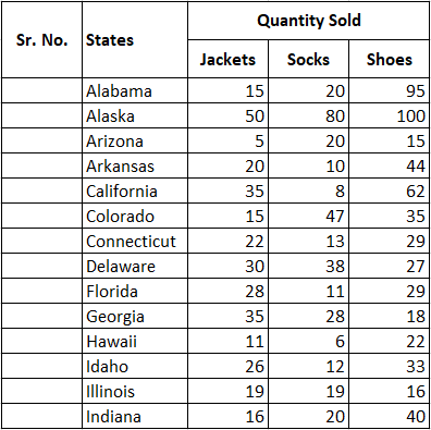
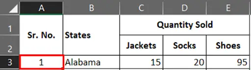
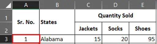
Suppose we have the following dataset and want to count the serial numbers.

Method 1 – Using Fill Handle

Step 1 – Enter Counting

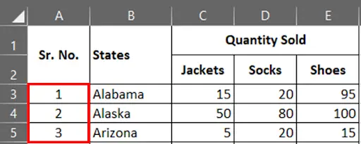
• In cell A3, A4 & A5 type 1, 2 & 3 respectively.

Step 2 – Select The Cells

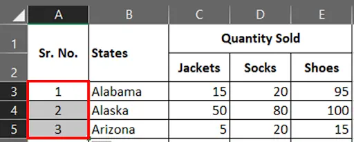
• Now select the cells from A3 to A5.
• Hover your mouse at the bottom right corner of cell A5, your cursor will change to a plus icon.

Step 3 – Double Click On The Selection

• While your cursor is in the  plus icon shape, double click on the selection. It will automatically fill in the serial numbers until the last data.

Method 2 – Using Fill Series

For this method, you must first count the number of records in your data. In our dataset, we have 14 US states. We will be using this in step 3.

Step 1 – Type 1

• Type 1 in cell A3.

Step 2 – Go To The Home Tab

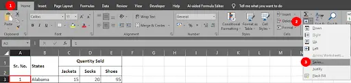
• While keeping the cursor at cell A3. Go to the Home Tab.
• Under the Editing group, click on the Fill dropdown button and select the Fill Series option.
• Series dialog box will appear on your screen.

Step 3 – Series Dialog Box

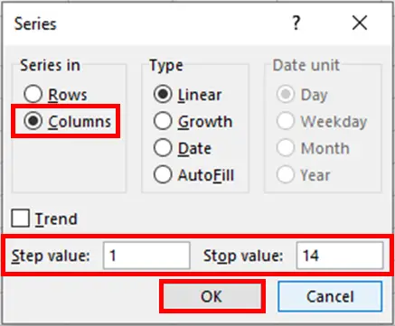
• In the series dialog box, under the Series In section, choose the column option.
• Value 1 is placed as the step value by default. Type the stop value and click the OK button.

Step 4 – Row Numbers Added

• By performing the above steps, you can easily fill in the serial numbers.

Method 3 – Add 1 To The Previous Number

Step 1 – Type Number 1

• In cell A3, type 1.

Step 2 – Enter The Formula

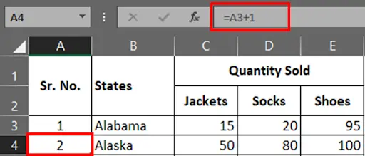
• In cell A4, enter the formula =A3+1 & press enter.

Step 3 – Drag The Formula

• Now drag the formula using the selection handle or copy and paste the formula down below the cells.

Method 4 – Using Array Formula

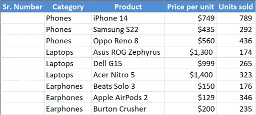
For this method, we will use the following dataset.

Step 1 – Select The Cell Range

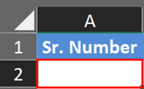
• Select the cell range where you want to type the formula. For our example, it’s A2:A49.

Step 2 – Type The Formula

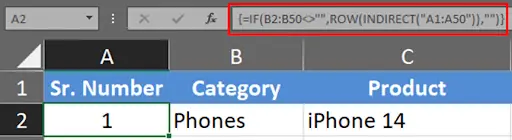
• We are going to use an array formula for this therefore, select all the cells in the range where you wish to apply the formula, then type the following formula in cell first cell i.e., A2..
• =IF(B2:B50<>””,ROW(INDIRECT(“A1:A50″)),””)
• As we are working with an array formula, press CTRL + SHIFT + ENTER to enter the formula.

Step 3 – Serial Numbers Added To The Dataset

• The serial numbers will be added to your dataset.

Formula Breakdown

=IF(B2:B50<>””,ROW(INDIRECT(“A1:A50″)),””)

The function above is an Excel formula that uses the IF statement to check if cells B2 to B50 contain any values. If any of these cells contain a value, the formula returns the row number of the corresponding cell in column A. If none of the cells in B2 to B50 contain a value, the formula returns an empty string.

Here’s a breakdown of the different parts of the formula:

• IF: This is the logical function that checks whether a condition is true or false. In this case, the condition is whether cells B2 to B50 contain any values.
• B2:B50<>””: This is the condition that the IF statement checks. It uses the comparison operator “<>” to check whether each cell in the range B2 to B50 is not equal to an empty string. If any of the cells in this range contain a value, the condition is true.
• ROW(INDIRECT(“A1:A50”)): This is the value that the formula returns if the condition is true. It uses the ROW function to return the row number of each cell in the range A1 to A50. The INDIRECT function is used to convert the range A1:A50 into a reference that can be used by the ROW function.
• ‘”’: This is the value that the formula returns if the condition is false. It is simply an empty string, which means that the cell containing the formula will appear blank if none of the cells in B2 to B50 contain a value.