How to make every other line shaded in Excel

You can watch a video tutorial here.

You have a table of data and you would like to make every other line shaded to better differentiate between rows.

There are two ways to do this:

Option 1 – Using Conditional Formatting

Step 1 – Opening Conditional Formatting Window

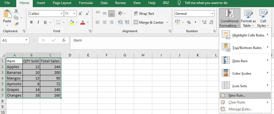
• Select the range that you want to format.
• In the Home Tab, click on Conditional Formatting in the Styles section.
• Select New Rule.

Step 2 – Setting up the Conditional Formatting formula

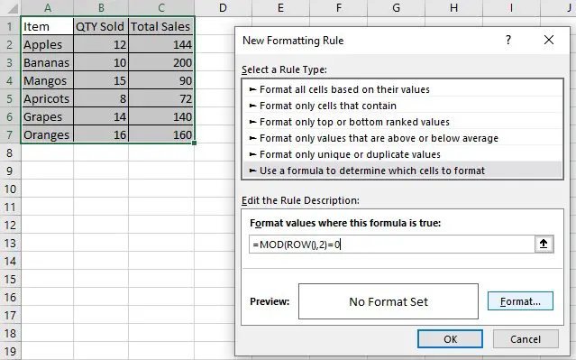
• Click on Use a formula to determine which cells to format.
• Type the following formula: =MOD(ROW(),2)=0.
• This rule uses a formula to determine whether a row is even or odd numbered.
• Select the Format button.

Step 3 – Setting up the Conditional Formatting format

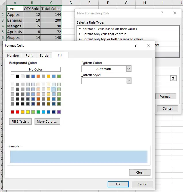
• Select the Fill tab and set the color you would like to highlight every second row with, as well as any other formatting you may wish for.
• Press OK.
• Press OK again.

Option 2 – Using the Format as Table function

Step 1 – Setting the Table Format

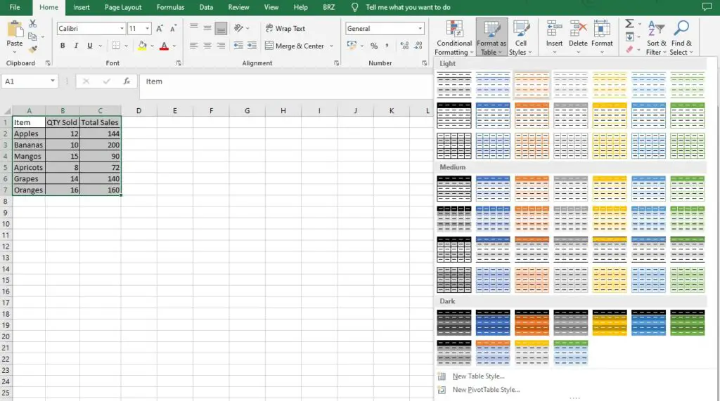
• Select the range that you want to format.
• In the Home Tab, click on Format as Table in the Styles section.
• Select whichever style you prefer.

Step 2 – Creating the Table

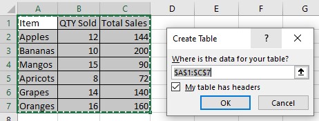
• Ensure that the range you want to format is selected.
• Tick the box if your table has headers.
• Click OK.

These are easy ways to make every other line shaded in Excel without using VBA.