How to make an ogive in Excel 

An ogive is a statistical graph that presents the cumulative frequency distribution of a dataset. It displays the cumulative frequencies below specific data points as a curved line. Ogives are utilized to summarize data concisely, calculate percentiles and quartiles, and facilitate comparisons between datasets. By visually representing the spread, concentration, and central tendency of the data. Ogives aid in analyzing and comprehending the dataset more effectively. 

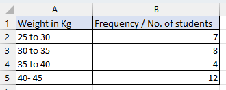
In this tutorial, we will use a dataset containing student weights and frequencies to create an ogive in Excel. Follow the steps below to learn how to generate an ogive graph using the given data, which will help visualize the cumulative frequency distribution. 

Method 1 – Cumulative Frequency Line Chart 

Step 1 – Create columns 

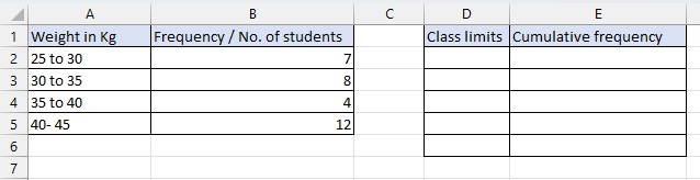
• Create two separate columns for cumulative frequency and class limits. 

Step 2 – Fill the data in the class limits column  

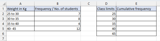
• Fill the class limits cell by entering the values starting from 25 till  45, make sure not to repeat any value. 

Step 3 – Fill the cumulative frequency column  

• To find cumulative frequency use the formula =SUM($B$2:B2). 
• Press enter. 
• Select the cell. 

• Move your cursor to the bottom right corner of the selected cell until it turns into a small black “+” sign. 
• Click and drag the cursor down or across the range of cells where you want to apply the formula. 

Step 4 – Insert an ogive graph 

• Select the cells.  
• Go to the Insert tab in the menu bar. 

• You will see different types of charts in the middle of the ribbon. 
• Select the scatter chart. 

Method 2 – Making an ogive using VBA code 

Step 1 – Open the VBA editor  

• Go to the “Developer” tab on the Excel ribbon. 
• Click on the “Visual Basic” button. 
• You can also press “Alt + F11” on your keyboard. This shortcut will directly open the (VBA) editor. 

• A window for the VBA editor will open. 

Step 2 – Insert a new module 

• In the VBA editor window, you will see the Project Explorer pane on the left-hand side. If it’s not visible, you can enable it by pressing “Ctrl + R” or going to the “View” menu and selecting “Project Explorer.” 
• In the Project Explorer, locate the workbook where you want to insert the module. Double-click on it to expand its contents. 
• Right-click on the workbook name or any existing module, and from the context menu, select “Insert” and then “Module. 
• A new module will be inserted into the workbook. It will appear as a separate module item under the workbook in the Project Explorer pane. 
• Another method to insert a new module is by clicking on the Insert menu at the top  

• Select the module option and a new module will appear separately under the workbook in the Project Explorer pane. 

Step 3 – Write the macro  

• Copy and paste the following macro  

Sub CreateOgive() 
    Dim ws As Worksheet 
    Dim chartObj As ChartObject 
    Dim chartDataRange As Range 
    Dim chart As chart 
     
    ‘ Set the worksheet where the data is located 
    Set ws = ThisWorkbook.Worksheets(“Sheet1”) ‘ Update the sheet name as needed 
     
    ‘ Set the range for the chart data 
    Set chartDataRange = ws.Range(“D1:E6”) 
     
    ‘ Add a new chart object to the worksheet 
    Set chartObj = ws.ChartObjects.Add(Left:=100, Top:=100, Width:=500, Height:=300) 
     
    ‘ Set the chart to the newly created chart object 
    Set chart = chartObj.chart 
     
    ‘ Set chart type to XY scatter with lines and markers 
    chart.ChartType = xlXYScatterLines 
     
    ‘ Set the source data range for the chart 
    chart.SetSourceData Source:=chartDataRange 
     
    ‘ Adjust chart properties as needed 
    With chart 
        .HasTitle = True 
        .ChartTitle.Text = “Ogive” 
        .Axes(xlCategory, xlPrimary).HasTitle = True 
        .Axes(xlCategory, xlPrimary).AxisTitle.Text = “Class limits” 
        .Axes(xlValue, xlPrimary).HasTitle = True 
        .Axes(xlValue, xlPrimary).AxisTitle.Text = “Cumulative frequency” 
    End With 
End Sub 

• After writing the code, close the VBA editor by clicking the “X” button or pressing “Alt + Q. 

Step 4 – Run the macro 

• Go to the “Developer” tab on the Excel ribbon and click on the “Macros” button in the “Code” group. 
• Select the Macro. 
• Click on Run. This will run the macro and an ogive will be inserted as shown below.