
How to make an interactive calendar in Excel 2020
 By
SpreadCheaters
By
SpreadCheaters

Making an interactive calendar in Excel 2020 typically involves creating a calendar grid with days, weeks, and months, adding interactive features that allow you to highlight specific dates or ranges, and navigating through the calendar. An interactive calendar in Excel 2020 allows users to view and manage dates and appointments easily, and track schedules and deadlines.
Step 1 – Form a Table for a Calendar
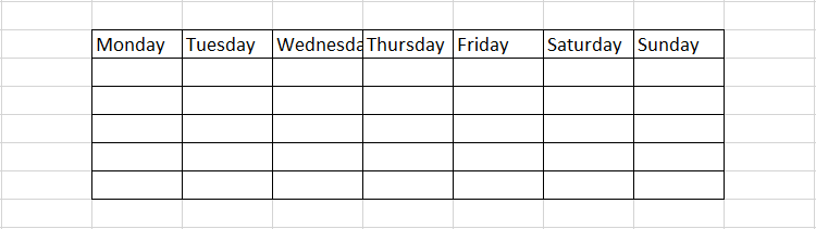
– Form a table for a calendar by typing the name of days in a row
– And make the border around it by clicking on All Borders from the drop-down list of border options in the Font group of the Home tab
Step 2 – Create a table for Month and Year
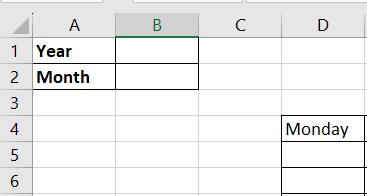
– After forming the table for the calendar, form a table for month and year
Step 3 – Type the name of the months
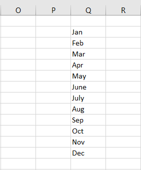
– After making the second table, type the name of the months in a column
Step 4 – Select the cell for Month
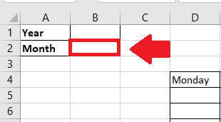
– Click on the cell where you want to show the months
Step 5 – Click on the Data Validation option
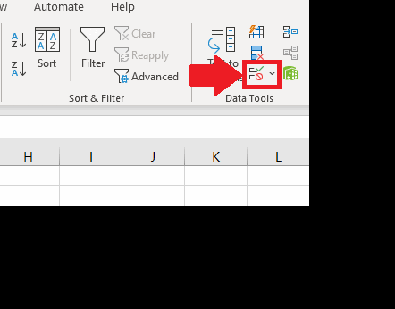
– After selecting the cell, click on the Data Validation option in the Data Tools group of the Data tab, and a dialog box will appear
Step 6 – Fill the dialog box
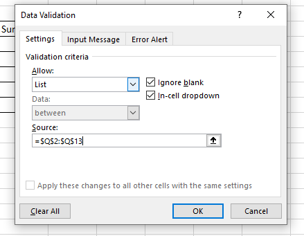
– Select the list in the box above the Allow option
– In the box above the Source option, type the range of cells containing the names of months(i.e Q2:Q13)
Step 7 – Click on Ok
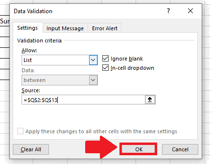
– After filling in the dialog box, click on OK to get the list in the selected cell
Step 8 – Make a table for 1st day and month number
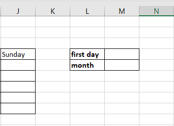
– Make another table containing the first day of the month and the number of months
Step 9 – Type the formula for the First day
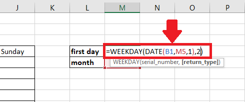
– In the cell next to the first day in the table type the formula :
– =WEEKDAY(DATE(B1,M5,1),2)
– Where B1 is the address of the cell containing the year
– Where M5 is the address of the cell containing the number of months
– Where 1 shows the first day of the month
– Where 2 shows that in counting the days of a week Monday is considered the first day of the week
Step 10 – Type the formula for the month number in the table
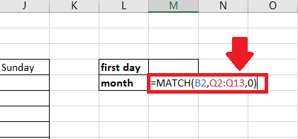
– After typing the formula for 1st day, type the formula for the month:
– =MATCH(B2,Q2:Q13,0)
– Where B2 is the cell address containing the list of names of months
– Where Q2:Q3 is the range of cells containing the names of months
– Where 0 shows the Exact match
Step 11 – Select the first cell of the calendar table
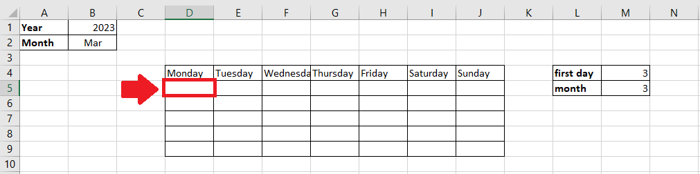
– Click on the first cell of the table that will show the calendar
Step 12 – Type the IF formula
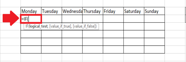
– In the selected cell, type the If formula
Step 13 – Type the first Argument of the IF function
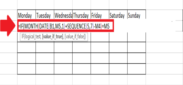
– First argument(Logical-Test) of IF function:
=IF(MONTH(DATE(B1,M5,1)+SEQUENCE(5,7)-M4)=M5
– MONTH: The MONTH function extracts the month number from a given date.
– The DATE function extracts days from the date. The date function requires three arguments i.e. B1 is the cell reference containing the year, M5 is the cell reference that contains the month, and 1 is the static value representing the day, in this case, it is the first day of the month.
– The SEQUENCE function generates an array of numbers in a specified range. The sequence function requires two arguments i.e. 5 is the number of rows in the generated array, and 7 is the number of columns in the generated array.
– M4 is a cell reference that contains a value representing the day of the week for the first day of the month M5 is a cell reference that contains the month value.
– The formula checks whether the month number obtained from adding the SEQUENCE array to the first day of the month (specified by the DATE function) is equal to the month number specified in the M5 cell.
Step 14 – Type the second argument of the IF function
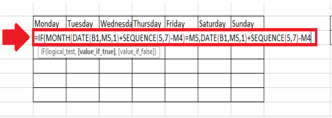
– The second argument of the IF function (Value if true) is followed when the condition is true:
– DATE(B1,M5,1)+SEQUENCE(5,7)-M4
The formula creates a date by combining the year value from the B1 cell, the month value from the M5 cell, and a day value of 1. This represents the first day of the month. The SEQUENCE function generates an array of numbers with 5 rows and 7 columns, which creates a 5×7 matrix of numbers from 1 to 35. The resulting array is added to the date value generated by the DATE function, resulting in a matrix of dates for the entire month.
Step 15 – Type the Third argument of the IF function
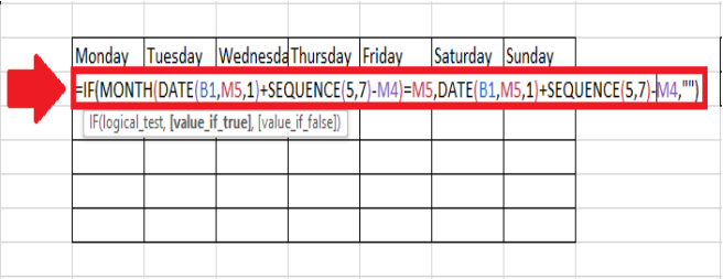
– The third argument of the IF function(Value if False) is:
– “”
It shows that if the condition is not true in the cell, then it will be left empty
Step 16 – Press the Enter key
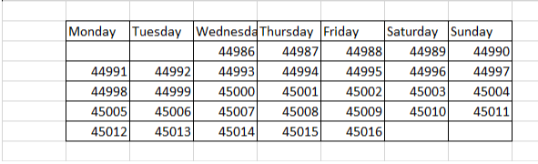
– After typing the third argument of the IF function, press the Enter key to get the calendar table in the form of numbers
Step 17 – Convert numbers into Date
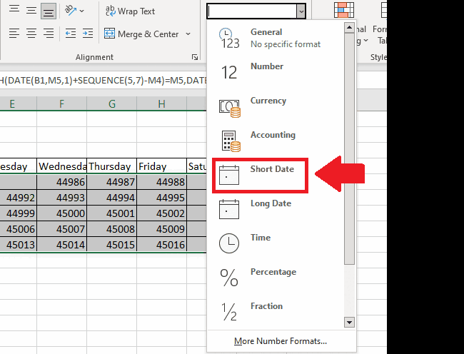
– Select the range of cells
– Click on the Number format option in the numbers group of the Home tab and a drop-down menu will appear
– From the drop-down menu, click on the Short Date option and the numbers will be changed to the date format
Step 18 – Click on the Number format option
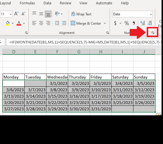
– Select the range of cells
– Click on the Number format option in the Numbers group of the Home tab and a dialog box will appear
Step 19 – Click on The Custom option

– In the dialog box, from the menu on the left side click on custom, and a new dialog box will appear
Step 20 – Change the Date format
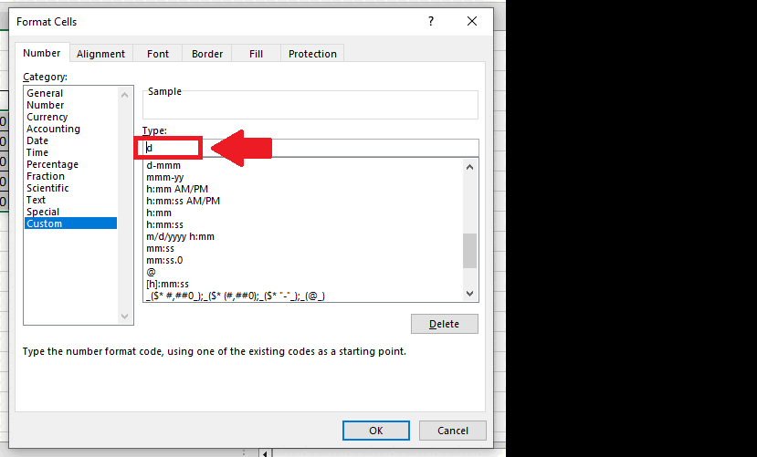
– Type “d” in the box below the type option (i.e only date)
– Click on OK to get the required calendar table
Step 21 – Get the Result
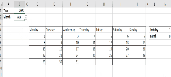
– Now you can change the date and year from the first table to get the calendar of that month and year


