
How to make all numbers negative in Excel
 By
SpreadCheaters
By
SpreadCheaters
To make all numbers negative in Excel means to convert all positive numbers in a given range or column to their negative equivalent. This can be useful for a variety of reasons, such as when you want to highlight losses or negative values in your data, or when you need to perform calculations that require negative numbers.
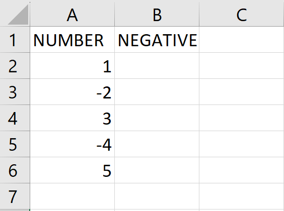
In this tutorial, we will learn how to make all numbers negative in excel. Our dataset contains different numbers(positive and negative), and we need to convert them to negative values. To do this, we have two methods, the first method is by using the IF function and the second is by using the ABS function. The following steps will guide you to use the IF function.
Method 1: Using IF function to convert numbers to negative
IF function is one of the logical functions, to return one value if a condition is true and another if it’s false. Syntax of IF function is:
=IF(logical_test, value_if_true, value_if_false)
The function uses the following arguments:
- Logical_test (required argument): This condition is tested and evaluated as either TRUE or FALSE.
- Value_if_true (optional argument): The value that will be returned if the logical_test evaluates to TRUE.
- Value_if_false (optional argument): The value that will be returned if the logical_test evaluates to FALSE
Step 1 – Select a cell
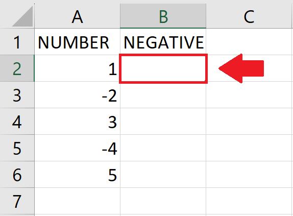
- Click on the cell where you want the negative number
Step 2 – Use The IF function
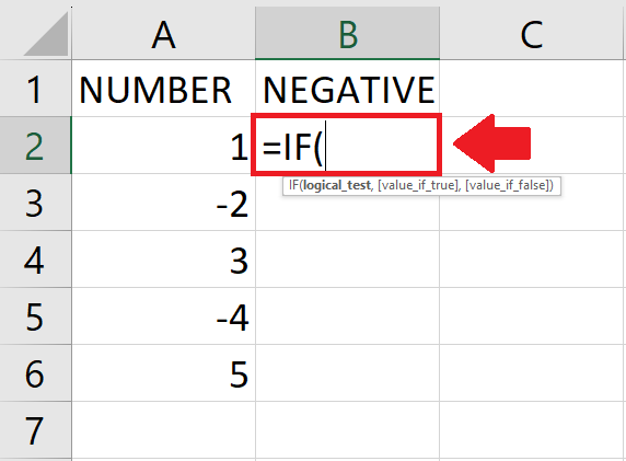
- To use IF function, type “ =IF(” in the selected cell
Step 3 – Type the Arguments
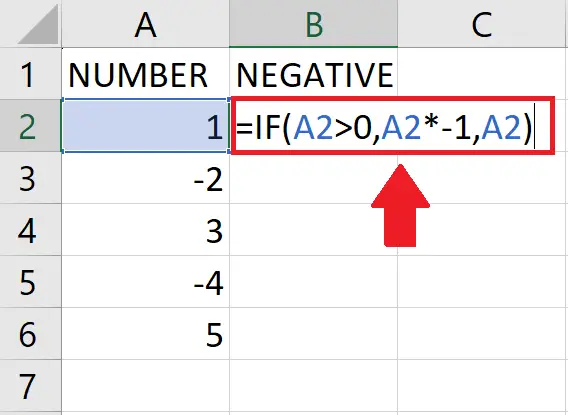
- Type the arguments of the IF function as shown below:
- Logical_Test: A2>0
- Value_if_true: A2*-1
- Value_if_false: A2
- After typing the arguments, type a closing bracket “)”
Step 4 – Press Enter Key
- After typing the arguments, press enter key to get the required result
Step 5 – Apply on the Entire Column
- After getting the result in the selected cell, use autofill to apply the IF function to the entire column
Method 2: Make all number negative using the negative ABS function
The ABS function in Excel is a mathematical function that returns the absolute value of a number.It’s Syntax is:
=ABS(number)
- The ABS function in Excel takes one argument, which is the number for which you want to calculate the absolute value. The argument can be a number or a reference to a cell that contains a number.
Step 1 – Select the cell
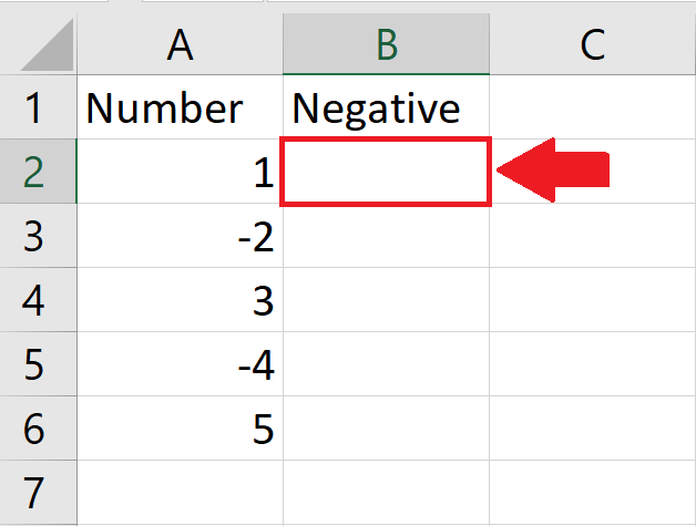
- Click on the cell where you want to show the negative value
Step 2 – Use the ABS function with negative sign
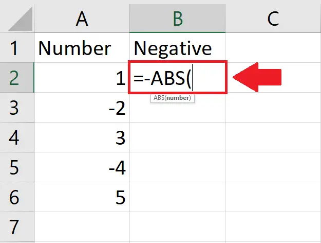
- Type “= -ABS(” in the selected cell to use negative ABS function
Step 3 – Type the Argument of the function
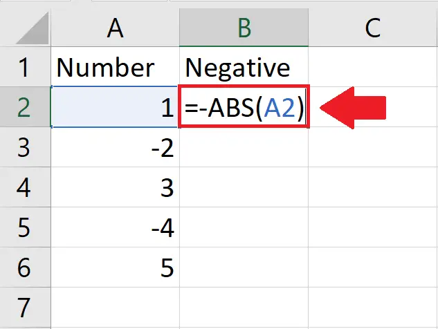
- After typing the Function, type it’s argument:
- Number: A2
- After typing the argument, type a closing bracket “)”
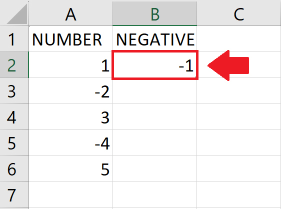
Step 4 – Press the Enter key
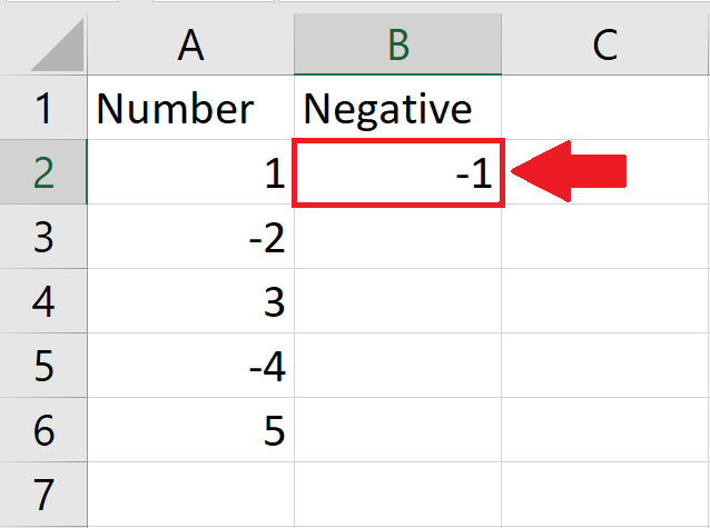
- After typing the arguments, press Enter key to get the required result
Step 5 – Apply the Function on Complete column
- After getting the result for the first cell, use autofill method to apply the function on complete column


