
How to make a tracker in Excel
 By
SpreadCheaters
By
SpreadCheaters
Our dataset comprises tasks assigned to students, including their ID, due date, and completion status. To generate a report from this dataset, we will create individual columns for each attribute. We will then apply conditional formatting to color-code the incomplete tasks and bring them to the top of the column for better visibility and emphasis.
Making a tracker in Excel refers to creating a spreadsheet that helps you organize, analyze, and track data. It typically involves creating columns and rows to input and manipulate data. It can enhance efficiency, accuracy, and decision-making in various personal, academic, and professional contexts.
Step 1 – Make a Column of the ID of the Tasks
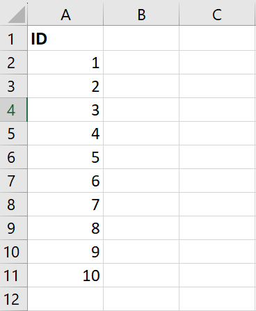
– Make a column in which you enter the ID of the tasks
Step 2 – Make a Column for the Task
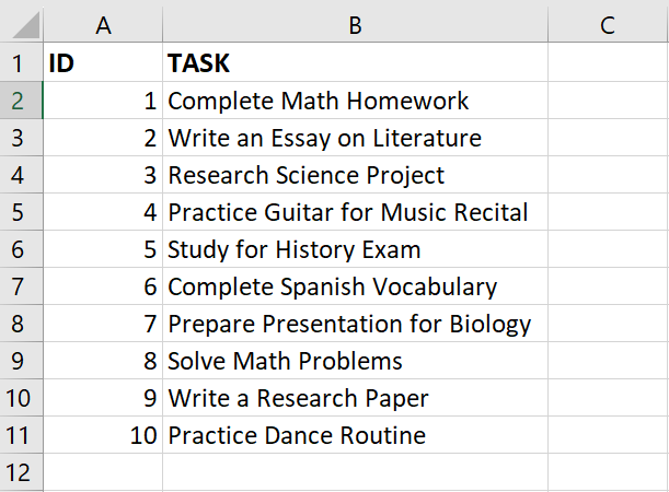
– After making the column of the ID, make a column consisting of the tasks i.e, name of tasks
Step 3 – Make a Column of Due date
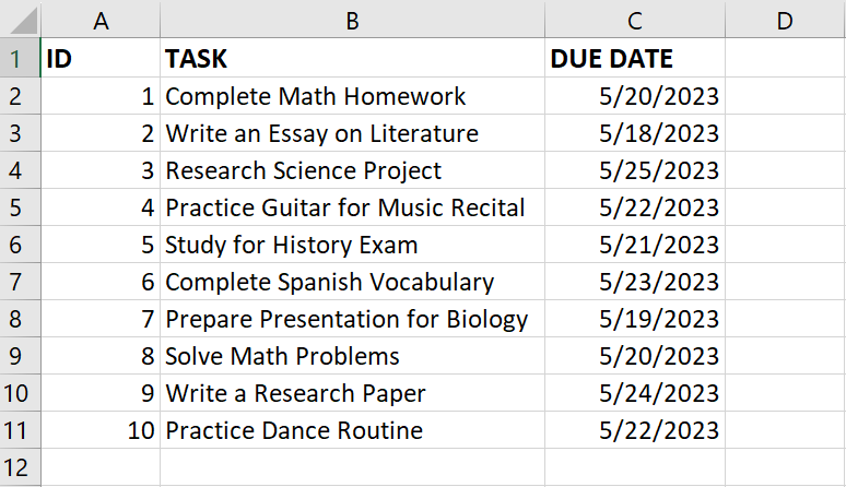
– Make a column for the due date containing the last date of every task
Step 4 – Make a Column of Status
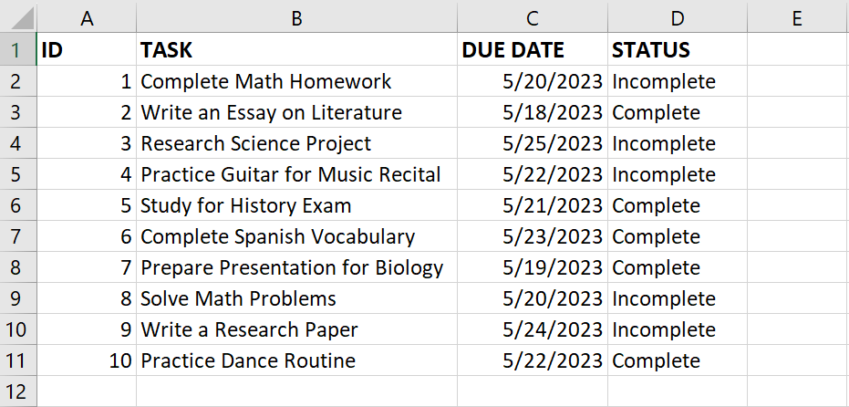
– After making the column of the due date, make a column having the status of each task i.e, either task is completed or not completed
Step 5 – Click on the Conditional Formatting option
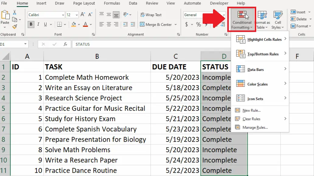
– After making the Status column, select this column
– Click on the Conditional Formatting option and a dropdown menu will appear
Step 6 – Click on the Highlight Cell rules option
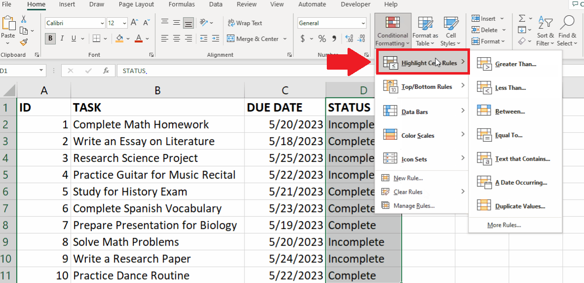
– Click on the Highlight Cell rules option in the dropdown menu, and a right-side menu will appear
Step 7 – Click on the Equal To option
– Click on the Equal To option in the right-side menu and a dialog box will appear
Step 8 – Select the Value
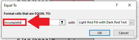
– Type Not Completed in the box below the Format cell Equal to option in the dialog box
Step 9 – Select the Colour
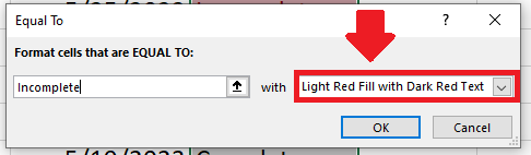
– Select the color in the box next to With the option
– Here we selected red color, you may select any other color you want
Step 10 – Click on OK
– After selecting the color, click on OK and the column containing the selected data will be colored
Step 11 – Click on the Sort and Filter option
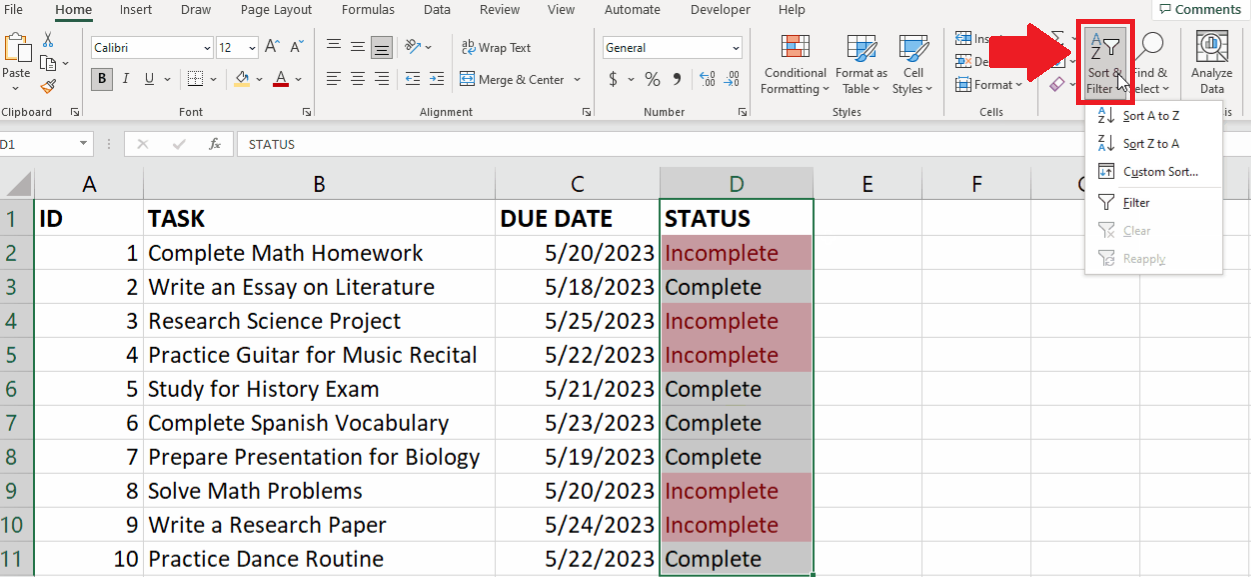
– After the cell got colored, select the status column
– Then click on the Sort and Filter option and a dialog box will appear
Step 12 – Click on the Custom Sort option
– Click on the Custom Sort option in the dropdown menu and a dialog box will appear
Step 13 – Select the Column
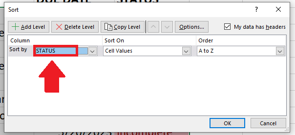
– Select the column, based on which you want to sort your data
– Here we have selected STATUS you may select any other as you want
Step 14 – Select the Cell Color option
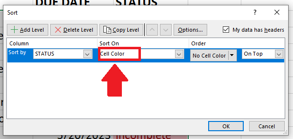
– Click on the Cell Color option in the box below the Sort on ion
Step 15 – Select the Color
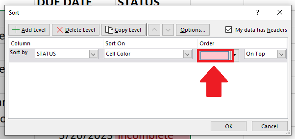
– Select the red color in the box below the Order option, to make all red-colored cells at the top of the column
Step 16 – Click on OK
– After selecting the color, click on OK to get the required result.
Conclusion:
By creating a task list, conditional formatting, and sorting the data in a useful way you can easily create a task tracker for your daily tasks. This approach can be extended to create more sophisticated task trackers which can be shared with colleagues or teammates to keep track of the status of project activities and timelines.


