How to lock the header in Excel

In this tutorial, we will learn how to lock the header in Excel. In Excel, locking the header means freezing the top row(s) and/or the left column(s) of a worksheet to remain visible as you scroll through the data. When you lock the header, you can easily refer to the row or column headers without manually scrolling back to the top of the worksheet, which can be especially helpful when working with a large amount of data.

Our dataset includes the schedule for a complete week, with the first column containing the days of the week and the remaining columns containing different times of the day. To enable scrolling while keeping the headers in place, we can use the “Freeze Panes” option to freeze the headers in their original positions.

Method 1: Lock the Row header

Step 1 – Select the Row

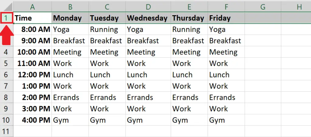
• Select the row that you want to lock by clicking on the row header
• You may select more than one row

Step 2 – Click on the Freeze Panes option

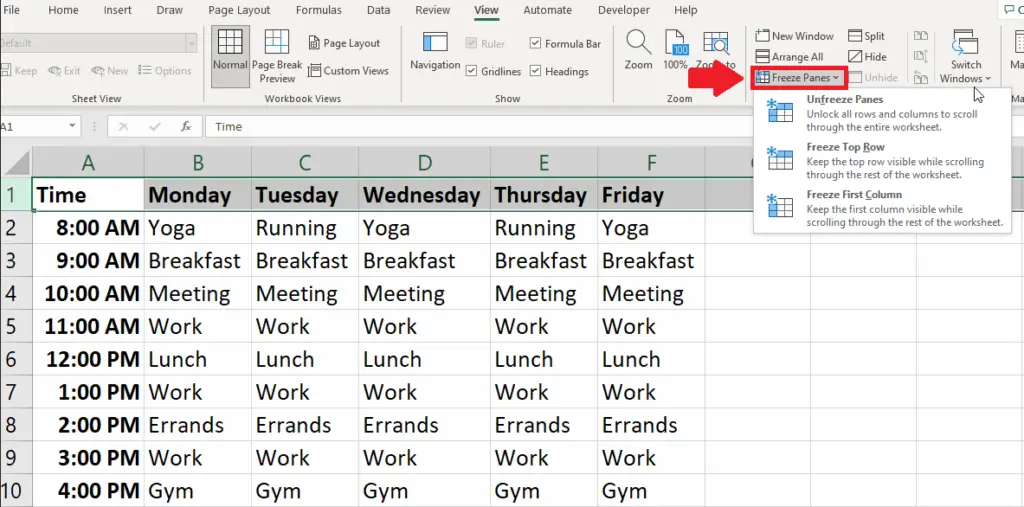
• After selecting the rows, click on the Freeze Panes option in the Windows group of the View tab  and a dropdown menu will appear

Step 3 – Click on the Freeze Top row option

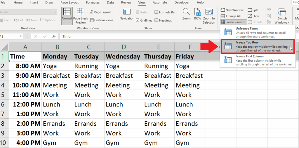
• From the drop-down menu, click on the Freeze Top row option

Step 4 – Get the Result

• After clicking on the Freeze top row option, scroll the sheet down to view the result

Method 2:  Lock the Column header

Step 1 – Select the Column

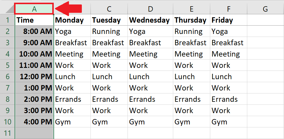
• Select the column that you want to lock by clicking on the row header
• You may select more than one column

Step 2 – Click on the Freeze Panes option

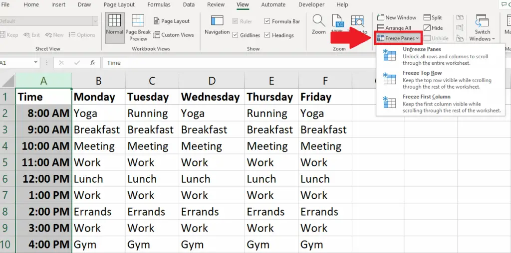
• After selecting the rows, click on the Freeze Panes option in the Windows group of the View tab and a dropdown menu will appear

Step 3 – Click on the Freeze First Column option

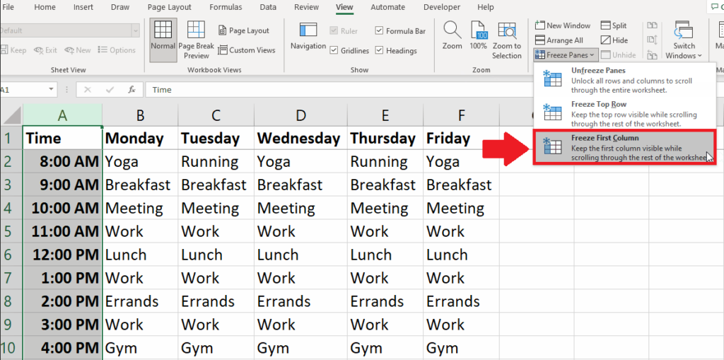
• From the drop-down menu, click on the Freeze  First Column option

Step 4 – Get the Result

• After clicking on the Freeze  First Column option, scroll the sheet left to view the result