How to lock only certain cells in Excel

Locking selected cells in Excel is a simple and effective way to safeguard important data, formulas, and structures in your spreadsheet. This feature allows you to specify which cells should be locked and which should be editable, providing a level of control and security over your data. Whether you’re working with sensitive financial information or a template that you want to protect from accidental changes, locking selected cells can help you maintain the accuracy and reliability of your spreadsheet.

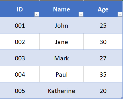
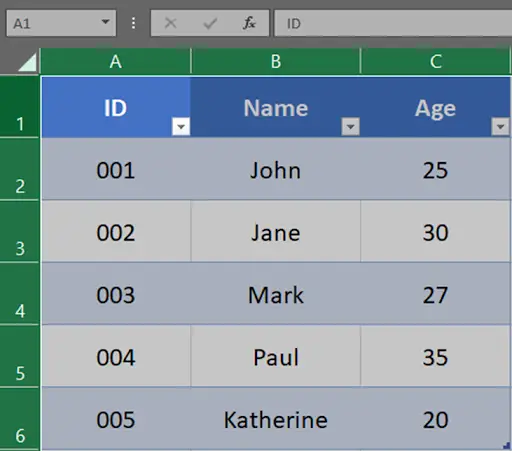
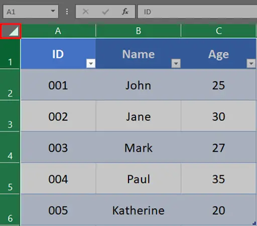
In this article, we’ll guide you through the process of locking selected cells in Excel with the following dataset shown above.

Locking all cells on an Excel sheet is easy, you just need to protect the sheet. Because the Locked attribute is selected for all cells by default, protecting the sheet automatically locks the cells.

If you don’t want to lock all cells on the sheet, but rather want to protect certain cells from overwriting, deleting or editing, you will need to unlock all cells first, then lock those specific cells, and then protect the sheet. To do this follow these steps. 

Method 1 – Using Context Menu 

Step 1 – Unlock All The Cells In The Sheet

• Click the select all button to select the entire sheet.

Step 2 – Open Format Cells Dialog Box

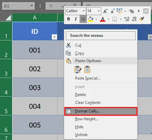
• Right click any of the selected cells & choose Format Cells from the context menu.

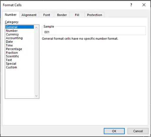
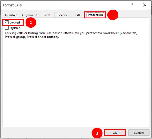
Step 3 – Format Cells Dialog Box

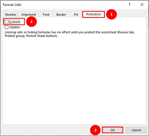
• In the Format Cells dialog, switch to the Protection Tab, un check the locked option and click OK.

Step 4 – Select Cells You Want To Lock

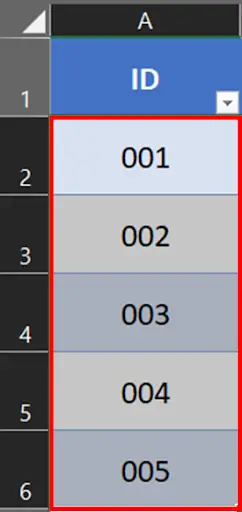
• For our example, we will lock cells in the ID column.
• Select them using mouse or arrow keys in combination with shift.

Step 5 – Open Format Cells Dialog Box

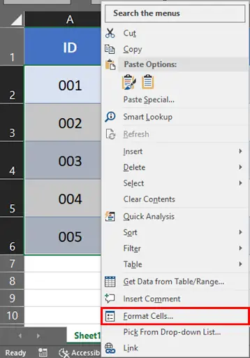
• Right click on the selected cells & choose Format Cells from the context menu.

Step 6 – Format Cells Dialog Box

• In the Format Cells dialog, switch to the Protection Tab, check the locked option and click OK.

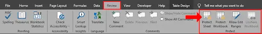
Step 7 – Protect The Sheet

• Locking Cells in excel has no effect until you protect the worksheet.
• To Protect the sheet. Click on the Review Tab, locate Protect group & click Protect Sheet button.

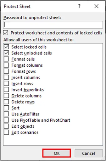
Step 8 – Protect Sheet Dialog Box

• You will be prompted to enter the password (optional).
• Select the actions you want to allow users to perform. Do this, & click OK.

Step 9 – Selected Cells Locked

• Done! The selected cells are locked and protected from any changes, while all other cells in the worksheet are editable.

Method 2 – Using Shortcut Key

Step 1 – Unlock All The Cells In The Sheet

• Press the short key CTRL + A to select the entire sheet.

Step 2 – Open Format Cells Dialog Box

• Press shortcut key CTRL + 1. Format cell dialog box will appear on your screen.

Step 3 – Format Cells Dialog Box

• Switch to the Protection Tab, un check the locked option and click OK.

Step 4 – Select Cells You Want To Lock

• To lock the cells in the ID column. Select them using mouse or arrow keys in combination with shift.

Step 5 – Open Format Cells Dialog Box

• Now, again press the shortcut key CTRL + 1. Format cell dialog box will appear on your screen. switch to the Protection Tab, check the locked option and click OK.

Step 6 – Protect The Sheet

• Locking Cells in excel has no effect until you protect the worksheet.
• To Protect the sheet. Click on the Review Tab, locate Protect group & click Protect Sheet button.

Step 7 – Protect Sheet Dialog Box

• You will be prompted to enter the password (optional).
• Select the actions you want to allow users to perform. Do this, & click OK.

Step 8 – Cells Locked & Protected

• The selected cells are locked and protected from any changes.

Method 3 – Using Number Group 

Step 1 – Unlock All The Cells In The Sheet

• Click the select all button to select the entire sheet.

Step 2 – Go To The Number Format Button

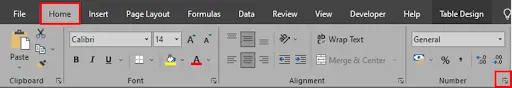
• Go to the Home Tab, in the Number Group click Number Format button.

Step 3 – Format Cells Dialog Box

• Switch to the Protection Tab, un check the locked option and click OK.

Step 4 – Select Cells You Want To Lock

• To lock the cells in the ID column. Select them using mouse or arrow keys in combination with shift.

Step 5 – Open Format Cells Dialog Box

• Now, again press the Number Format button. Format cell dialog box will appear on your screen. switch to the Protection Tab, check the locked option and click OK.

Step 6 – Protect The Sheet

• Locking Cells in excel has no effect until you protect the worksheet.
• To Protect the sheet. Click on the Review Tab, locate Protect group & click Protect Sheet button.

Step 7 – Protect Sheet Dialog Box

• You will be prompted to enter the password (optional).
• Select the actions you want to allow users to perform. Do this, & click OK.

Step 8 – Cells Locked & Protected

• The selected cells are locked and protected from any changes.