
How to label a legend in Microsoft Excel
 By
SpreadCheaters
By
SpreadCheaters
In this tutorial, we will learn how to label a legend in Microsoft Excel. In Microsoft Excel, it’s possible to label a legend or modify its label by using the Select Data button in the Chart Design tab.
Currently, we have a data set representing sales for the month of January in different regions. We want to label the legend i.e. “East January” as “East February”.
The legend in Excel refers to a key that provides information about the colours or symbols used in a chart or graph. Legends are essential in helping readers interpret and understand the data being presented in a visual format. With the ability to customize font styles and sizes, Excel legends can be easily formatted to fit the overall aesthetic of a document or presentation.
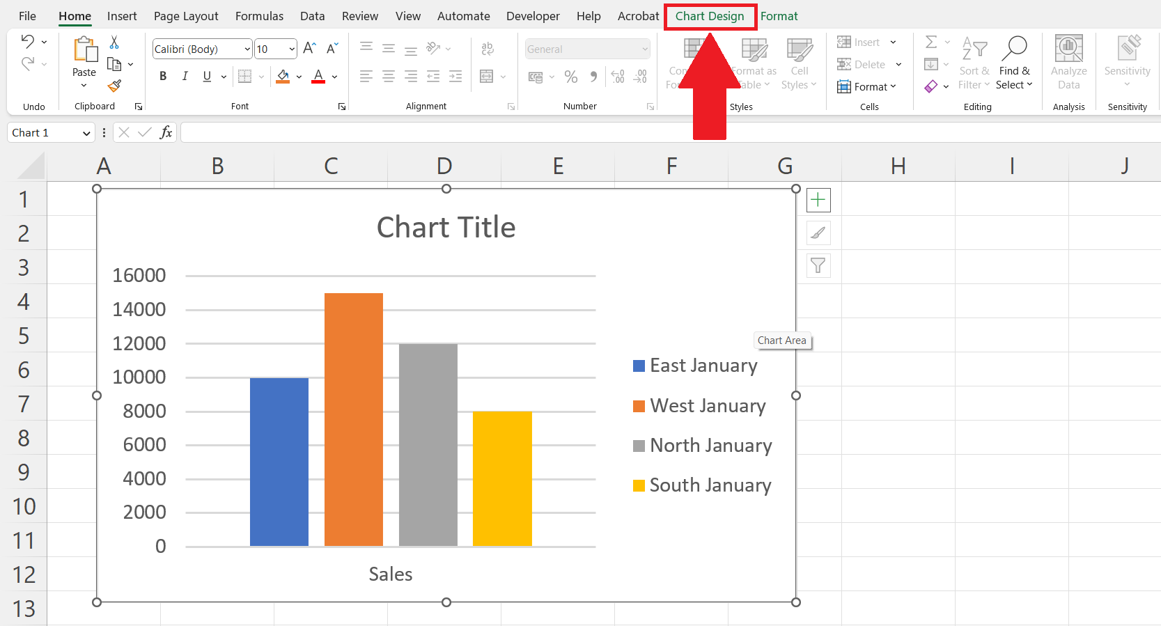
Step 1 – Click Anywhere on the Chart
– Click anywhere on the chart containing the legend to be labelled.
– A Chart Design tab will appear in the menu bar.
Step 2 – Go to the Chart Design Tab
– Go to the Chart Design tab in the menu bar.
Step 3 – Click on the Select Data button
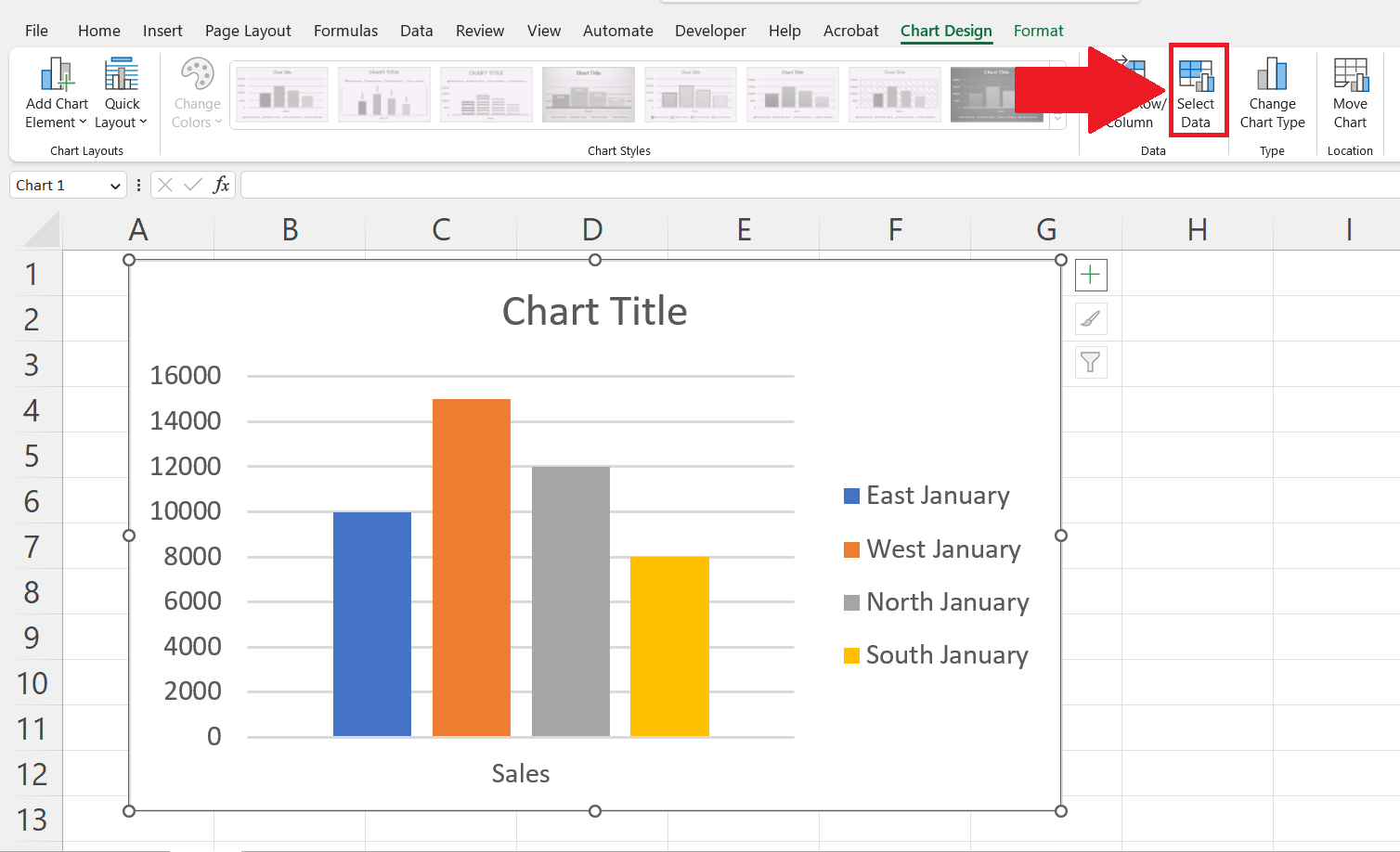
– Click on the Select Data button in the Data section of the Chart Design tab.
– A Select Data Source dialogue box will appear.
Step 4 – Select the Legend to be Labeled
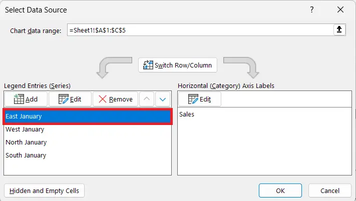
– Select the Legend to be labelled in the Legend Entries box.
Step 5 – Click on the Edit Button
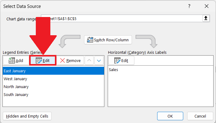
– Click on the Edit button.
– An Edit Series dialogue box will appear.
Step 6 – Label the Legend and Click on OK
– Label the legend in the series name option.
– Click on OK in the Edit Series dialogue box.
Step 7 – Click on OK

– Click on OK in the Select Data Source dialog box.
– The legend will be labeled.


