How to invert cells in Excel

Inverting cells” in Excel typically refers to reversing the order of the values in a selected range of cells. In general, inverting cells in Excel provides a quick and efficient way to reverse the order of data in a column or row, which can be useful in a variety of situations.

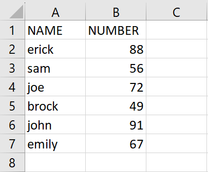
Our data set contains the names and marks of students, and we wish to invert the cells. We will explore three methods to achieve this: the first is by using the sort option, the second is by using the A to Z option and the third one is to use a combination of INDEX and ROW functions. The following steps will help you to use these options.

Method 1: Invert Cells using the Sort option

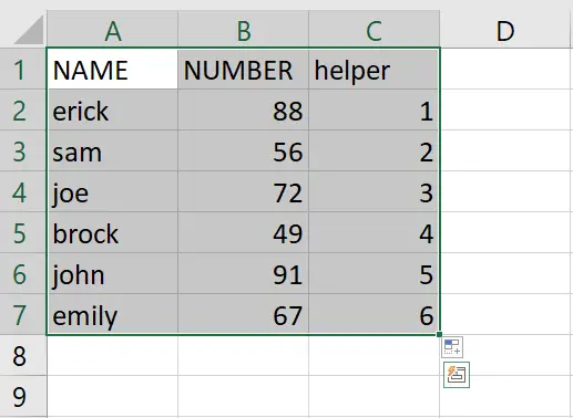
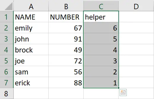
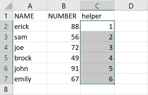
Step 1 – make a helper column

•  To make helper column type helper in the first cell of the column next to the (last column) of data to be flipped
• After typing helper, type 1,2,3 in the cells below it
• After typing 1,2.3, drag it till 3 then use Autofill(till the data to be flipped ends) to get the numbers in the complete column

Step 2 – Select the Range of Cells

• After typing the Helper column, select the range of cells including the data to be flipped, and the Helper column

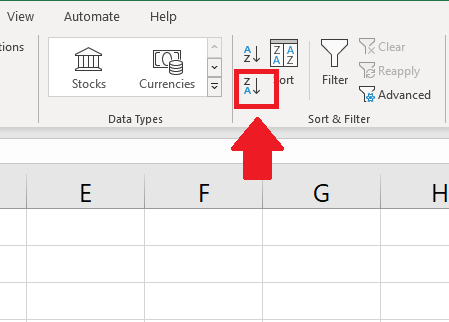
Step 3 – Click on the Sort option

• After selecting the range of cells, click on the Sort option from the Sort and Filter group of the Data tab

Step 4 – Select Helper as  the column to be sorted

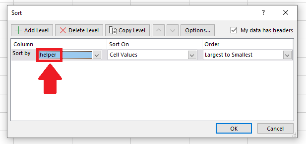
• In the dialog box, select helper as the column to be sorted in the box next to the Sort by option

Step 5 – Select the Largest to Smallest order

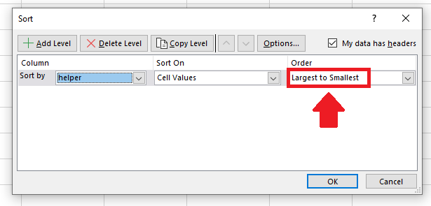
• In the dialog box, select Largest to smallest order in the box below the Order option

Step 6 – Click on Ok 

• After selecting the order, click on OK to invert the cells

Step 7 – Select the Helper Column

• After inverting the cells, select the Helper column

Step 8 – Delete the Helper Column

• After selecting the Helper column, delete it
• To Delete the column open the context menu(by right-clicking in the column)
• From the context menu, click on Delete and a dialog box will appear
• In the dialog box, click on the Entire column to get the required result

Method 2: Invert cells using A to Z option

Step 1 – make a helper column

•  To make helper column type helper in the first cell of the column next to the (last column) of data to be flipped
• After typing helper, type 1,2,3 in the cells below it
• After typing 1,2.3, drag it till 3 then use Autofill(till the data to be flipped ends) to get the numbers in the complete column

Step 2 – Select the Helper Column

• Select the helper column by drag and drop method

Step 3 – Click on the Z to A option

• After selecting the Helper row, Click on the Z to A option in the Sort and Filter group of the Data tab and a dropdown menu will appear

Step 4 – Click on the Expand the Selection option

• In the dialog box, click on the  Expand the Selection option 
• Click on Sort at the end of the dialog box to Invert the cells

Step 5 – Delete the Helper Column

• After selecting the Helper column, delete it
• To Delete the column open the context menu(by right-clicking in the column)
• From the context menu, click on Delete and a dialog box will appear
• In the dialog box, click on the Entire column to get the required result

Method 3 Invert the cells in a column using the formula

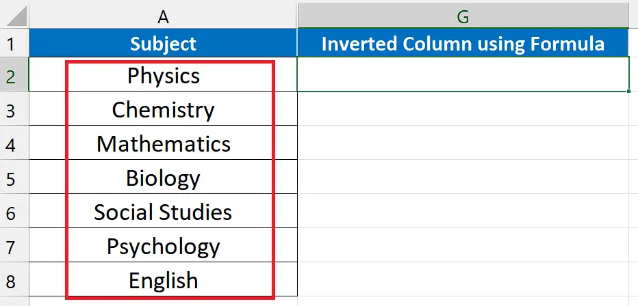
We can also use a generic formula to invert the cells of a column. The formula is fairly very simple and easy to understand as well. This formula involves using a combination of INDEX and ROWS functions. Let’s dive into a practical example and follow the steps mentioned below to learn this method. Our dataset contains the names of subjects in a random order as shown below. We’ll use the formula and invert the order of the column and place the new values in a new column.

Step 1 – Create the formula using INDEX & ROWS functions

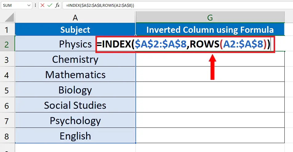
• Choose an appropriate cell that will be the starting cell of the inverted column and write down the following formula in that cell.

=INDEX($A$2:$A$8,ROWS(A2:$A$8))

Step 2 – Implement the formula to get the first result

• After writing the formula correctly, press the enter key to get the first result as shown above.

Step 3 – Implement the formula to invert the whole column

• Now hover the mouse cursor on the bottom right corner of the first cell in the inverted column.
• The mouse cursor will change to a black plus sign, which is called the fill handle. Double-click the mouse’s right button and you will get your data column inverted, as shown above.

Breakdown of the formula

The formula mainly utilizes the INDEX function, which retrieves an element’s value from an array based on specified row and column numbers. To implement the “flip column” trick, the array is set to the entire list that needs to be reversed, which is A2:A8 in this case. The ROWS function determines the row number, which essentially counts down from the array’s last row to the first row. This is accomplished by referencing the first row of the array with an absolute reference, and then using a relative reference to change the starting row as the formula is copied down. 

The resulting effect is that the INDEX function moves from the last element to the first element, with each iteration of the formula, based on the decrementing counter created by the ROWS function.