
How to implement markup formula in Microsoft Excel
 By
SpreadCheaters
By
SpreadCheaters
In this tutorial we will learn how to implement the Percentage Markup formula in Microsoft Excel. Markup formulas are mathematical expressions that calculate the amount by which the cost price of a product or service is increased to arrive at the selling price. The most commonly used markup formula in Excel to calculate selling price is (cost price x (1 + markup percentage)). This formula takes the cost price of a product or service and multiplies it by the markup percentage, which is then added to the cost price to arrive at the selling price.
Microsoft Excel is a spreadsheet software that allows users to organize, analyze, and manipulate data. It is widely used in various industries and is considered a valuable tool for data management, analysis, and presentation. Excel provides users with a wide range of features including calculation tools, pivot tables, charts and graphs, and macro programming capabilities.
Step 1 – Enter the Markup Percentages separately
– Enter the markup percentages in separate cells.
Step 2 – Select a blank cell
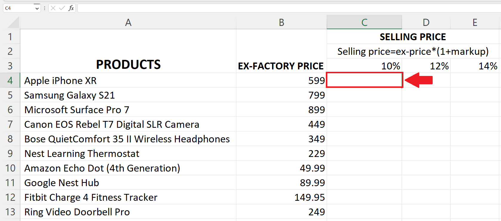
– Select a targeted cell where you want the selling price to be.
Step 3 – Place an Equals sign
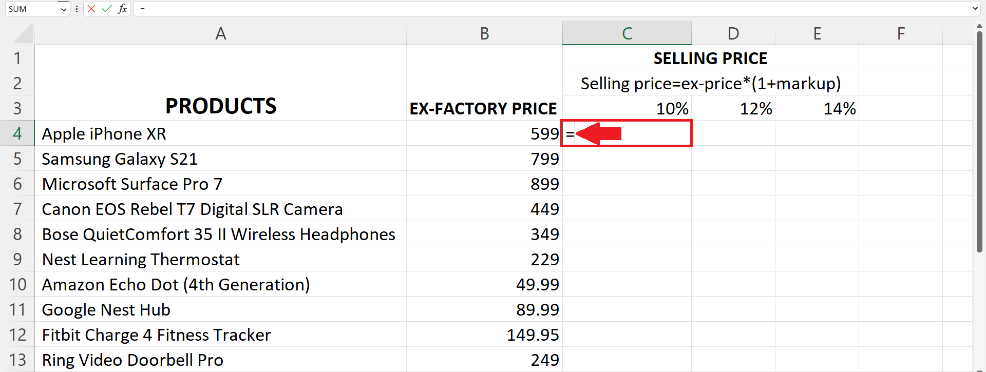
– Place an Equals sign (=) in the targeted cell.
Step 4 – Enter the Percentage Markup formula
– Enter the Percentage Markup formula in the cell i.e.
Ex-Price*(1+Markup)
– Where Ex-Price is the address of the cell containing Ex-Price and Markup is the address of the cell containing the markup percentage.
Step 5 – Use the “$” sign
– Place the “$” sign before the column of the Ex-Price cell address as it has to remain the same,only the row number will change.
– Place another “$” sign before the Row number of the Markup cell address since the row has to be the same and columns will change.
Step 6 – Press the Enter key
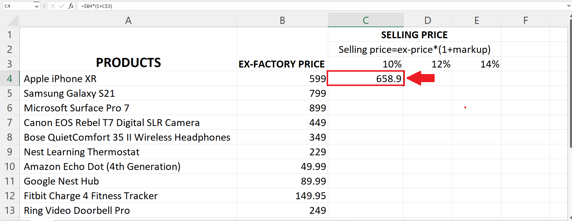
– Press the Enter key to get the results.
Step 7 – Use the Handle Select and Drag and Drop Method

– Use the “Handle Select” and “Drag and Drop” method to apply the Percentage Markup formula on each row and column.


