How to identify outliers in Excel

In Excel, an outlier is a data point that is significantly different from the rest of the data. Identifying outliers can help detect errors, anomalies, or unusual patterns in your data. Identifying outliers can also help in Quality Control, Statistical analysis, and  Machine learning.

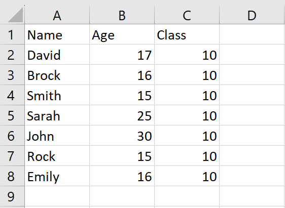
In this tutorial, we will learn. Our dataset above comprises information on students in Class 9, including their names, class, and ages. We aim to identify outliers based on age, for this we have two methods, the first is by using Sort and Filter and the second is by using the Quartile function. The following steps will guide you to use these methods.

Method 1: Using Sort and Filter

Step 1 – Select the range of cells

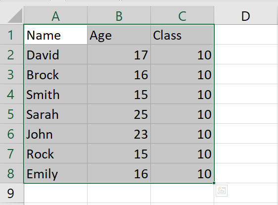
• Select the range of cells that contain outliers

Step 2 – Click on the Sort and Filter option

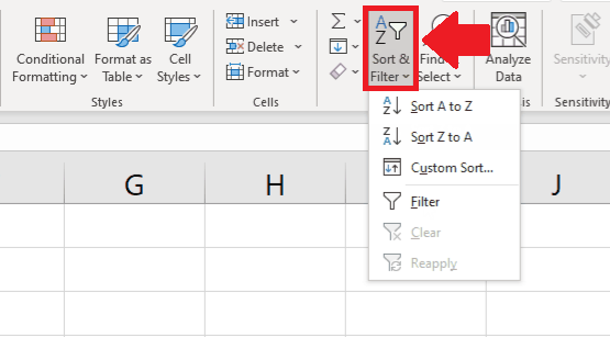
• After selecting the range of cells, click on the Sort and Filter option and a drop-down menu will appear

Step 3 – Click on the Custom Sort option

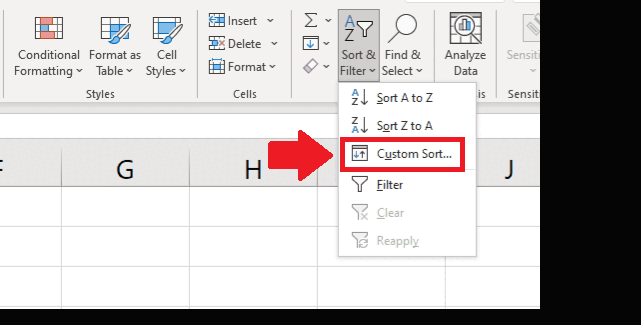
• From the drop-down menu, click on the  Custom Sort option and a dialog box will appear

Step 4 – Fill the Dialog box

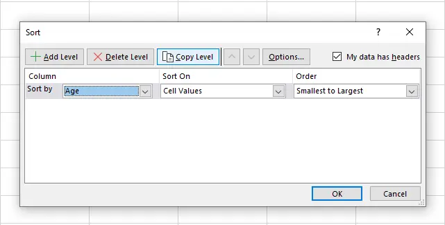
• Fill in the dialog box as follows:
• Column: Age
• Sort on: Cell Values
• Order: Smallest to Largest

Step 5 – Click on OK

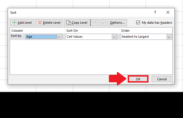
• After filling in the dialog box, click on OK at the end of the dialog box  to get the out liars at the end of the selected range 
• You may get the outliers at the top of the selected range 

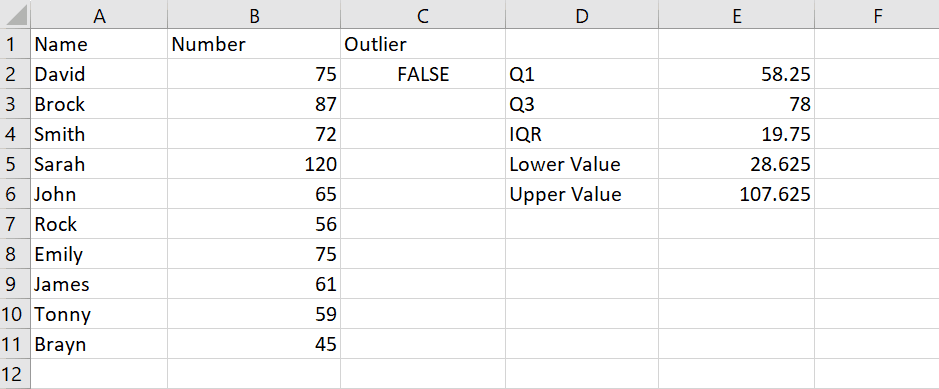
Method 2: Identify outliers using QUARTILE 

Step 1 – Type the Formula for Q1

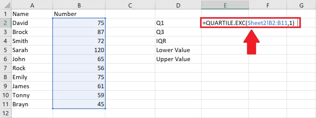
• Click on the cell where you want to show Q1
• Type the formula:
• =QUARTILE.EXC(Sheet2!B2:B11,1)  

Step 2 – Type the Formula for Q2

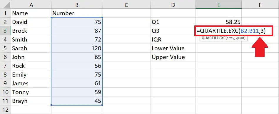
• Click on the cell where you want to show Q2
• Type the formula:
•  =QUARTILE.EXC(B2:B11,3)       

Step 3 – Type the Formula for IQR

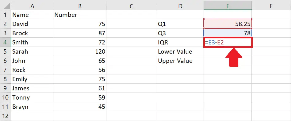
• Click on the cell where you want to show IQR
• Type the formula:
• =E2-E4

Step 4 – Type Formula for Lower Value

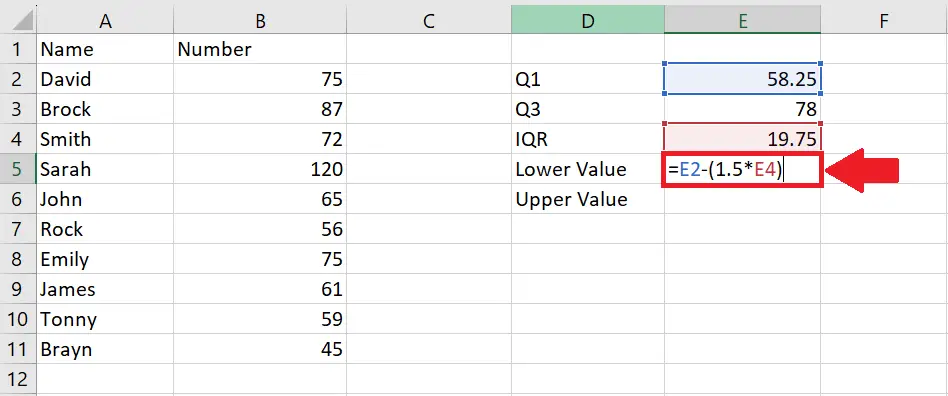
• Click on the cell where you want to show a lower value
• Type the formula:
• =E2-(1.5*E4)

Step 5 – Type the Formula for the Higher value 

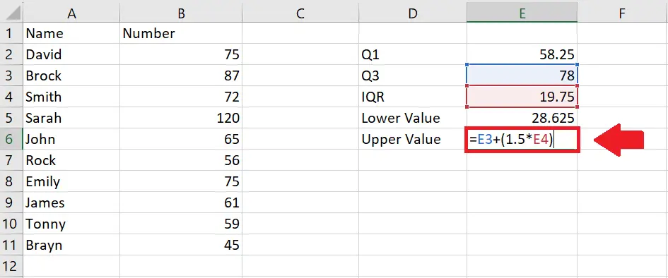
• Click on the cell where you want to show higher vale
• Type the formula:
• =E3+(1.5*E4)

Step 6 – Type the Formula to identify the Outliers

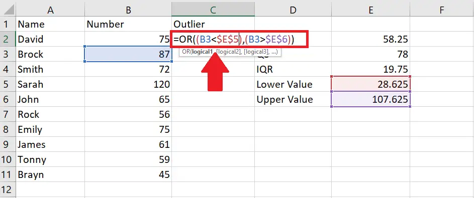
• Click on the cell where you want to identify the outlier
• Type the formula:
• =OR((B3<$E$5),(B3>$E$6))
• It will show TRUE against the cell having the value that is an outlier while FALSE for the value that is not an outlier

Step 7 – Apply the Formula to Complete the column

• After getting the result in the first cell
• Use the Autofill method to apply the effect on the complete column