How to highlight words in Excel 

When preparing Excel data for presentations or reports, highlighting text can enhance the visual appeal and professionalism of your materials. By using consistent and meaningful highlighting techniques, you can make your data more visually appealing and easier to comprehend for your audience. This can help in conveying key messages effectively and ensuring that important details are not overlooked.

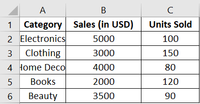
The “Sales Data” dataset provides information on sales performance across different categories for a company. It includes details such as the category name, total sales amount in USD, and the number of units sold within each category. Analyzing this dataset allows for insights into the performance of various product categories, aiding in decision-making related to resource allocation, marketing strategies, and product planning.

Method – 1 Highlighting cells from cell styles

The first and easiest method is to use the pre-defined cell highlighting styles which are available in the Styles Group of Home Tab. Let’s see how it can be done.

Step – 1 Go to Cell styles

• Open the Microsoft Excel document on your device, Select a cell you want to highlight.
• From the top menu, select Home and go to Cell Styles.

Step – 2 Highlight your text to your accordance 

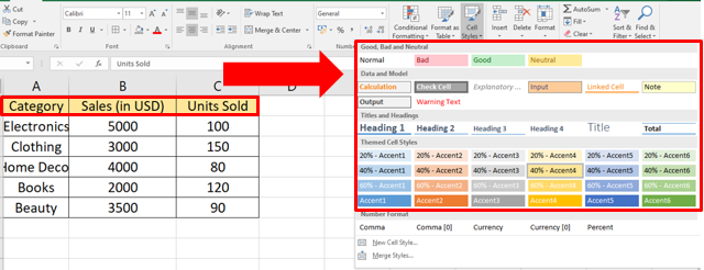
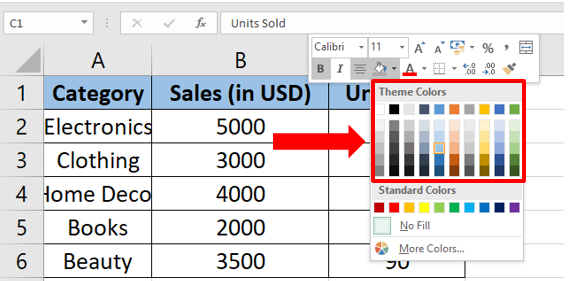
• A menu with a variety of cell color options pops up. Hover your mouse cursor over each color to see a live preview of the cell color change in the Excel file.
• When you find a highlight color that you like, select it to apply the change.

Method – 2 Highlighting text using context menu options

Secondly, the context menu options can also be used to highlight text as per your requirements. Follow the steps explained below to learn how to do it.

Step – 1 Left click on selected text 

• Open your Microsoft Excel document, double-click the cell containing text you want to format.
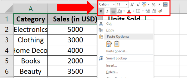
• Press the left mouse button and drag it across the words you want to colorize to highlight them. A small menu appears.

Step -2 Highlight text with your accordance 

• Select the Font Color icon in the small menu to use the default color option or select the arrow next to it to choose a custom color.
• Select a text color from the pop-up color palette the color is applied to the selected text. Select elsewhere in the Excel document to deselect the cell.

Method – 3 Highlight Text in Excel Using Conditional Formatting

Conditional formatting is an essential tool in Excel that allows you to easily identify and highlight specific data points based on user-defined criteria. By using conditional formatting to highlight text in Excel, you can quickly draw attention to important information and make your data more readable and understandable. This can be particularly helpful when dealing with large sets of data or complex spreadsheets where it may be difficult to identify important information at a glance. So, please follow the steps explained below to learn how to apply a simple case of conditional formatting to highlight the text.

Step – 1 Locate the “Text that Contains…” option in conditional formatting group

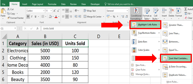
• Open your Microsoft Excel document, select the cells containing text you want to format.
• Then go to Home, in Conditional Formatting go to  Highlight Cells Rules select Text that contains

Step – 2 Highlight text with your accordance

• After clicking the Text that Contains command, you will see a dialog box pops up on the screen. 
• Within the box, Type texts based on which you want to format cells.
• For instance, we’ve typed “old”. This will highlight all the cells that contain the text old in them.
•  After that hit the OK button.

Conclusion:

Overall, highlighting text in Excel serves as a valuable tool for emphasizing important information, data validation, visualization, organization, and enhancing the overall readability and impact of your spreadsheets.