
How to Highlight Separate Columns in Excel
 By
SpreadCheaters
By
SpreadCheaters
If you work with spreadsheets regularly, you know how important it is to have a clear and organized view of your data. Highlighting separate columns in Excel is a great way to improve the readability and understanding of your data. Whether you want to highlight odd or even columns, or specific columns with certain data types, Excel offers a variety of formatting options to make your data stand out. In this article, we will show you how to highlight separate columns in Excel using easy-to-follow steps.
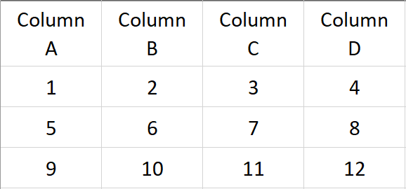
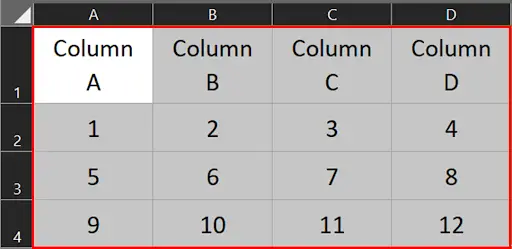
Suppose we have the following data & we want to highlight separate columns.
Method 1 – Manually Select Columns
Step 1 – Select Columns
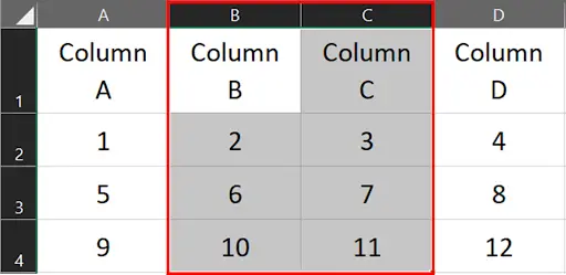
- Select the column(s) you want to highlight by clicking on the column letter(s).
Step 2 – Fill Colour Button
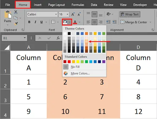
- Go to the Home Tab, in the Fonts group click on the Fill Colour button & select your desired colour.
Step 3 – Columns Highlighted
- This is the simple & quickest way to highlight the columns.
Method 2 – Highlight Columns Through Excel Table
Step 1 – Select Data

- Select your data.
Step 2 – Convert Data Into Table
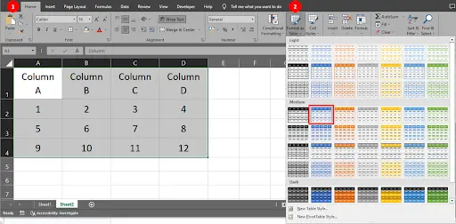
- To do this, go to the Styles group in the Home Tab & click Format As Tables button.
- Click on your desired table style.
Step 3 – Create Table Dialog Box
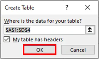
- Create table dialog box will appear on your screen.
- Click OK button. You data will be converted into Excel Table.
Step 4 – Table Styles Options
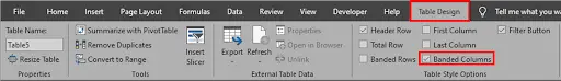
- Click anywhere on the table.
- Go to the Table Styles Options in the Table Design Tab.
- Uncheck the Banded rows option & check the Banded columns option.
Step 5 – Alternate Columns Highlighted
- Through this method, you can highlight alternate columns of your table.
Method 3 – Highlight Columns Through Conditional Formatting
Step 1 – Select Data
- Select your data.
Step 2 – Go To Conditional Formatting
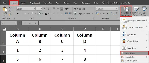
- At the Home Tab, in the Styles group click on the conditional formatting button & select New Rule.
Step 3 – New Formatting Rule
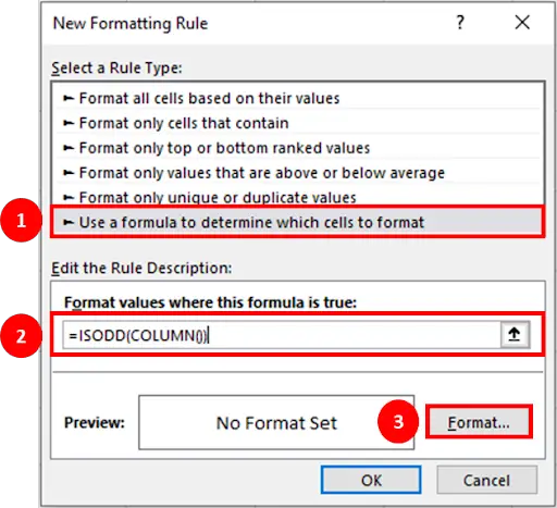
- New Formatting Rule dialog box will appear on your screen.
- Click on Use a formula to determine which cells to format option.
- Type the formula =ISODD(COLUMN()) in the edit rule description.
- Click the Format button to set cell formatting.
Step 4 – Set The Cell Formatting
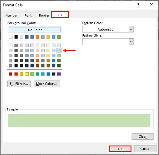
- Format Cells screen will appear on your screen.
- Click on the Fill tab, choose your desired colour & click the OK button.
Step 5 – Columns Highlighted
- Click OK on the new formatting rule screen. Odd numbered columns of your data will be highlighted.
Formula Breakup
The Excel formula =ISODD(COLUMN()) checks whether the column number of the cell in which the formula is written is odd or not.
The COLUMN() function returns the column number of the cell where the formula is placed. For example, if the formula is placed in cell A1, the COLUMN() function will return 1.
The ISODD() function then checks whether the column number returned by the COLUMN() function is odd or not. If the column number is odd, the formula will return the logical value TRUE, and if the column number is even, the formula will return FALSE.


