How to highlight selected cells in Excel

You can watch a video tutorial here.

Excel provides several options for formatting cells. You may want to draw the reader’s attention to particular pieces of information on a sheet by highlighting the cells. To do this, you can change the background color of the cell so that it stands out. 

Option 1 – Use the button on the ribbon

Step 1 – Select the cells

• Select the first cell to be highlighted
• Hold down the Ctrl key and click on the next cell
• Click on each of the cells to be highlighted, holding down the Ctrl key all the while

Step 2 – Choose a color

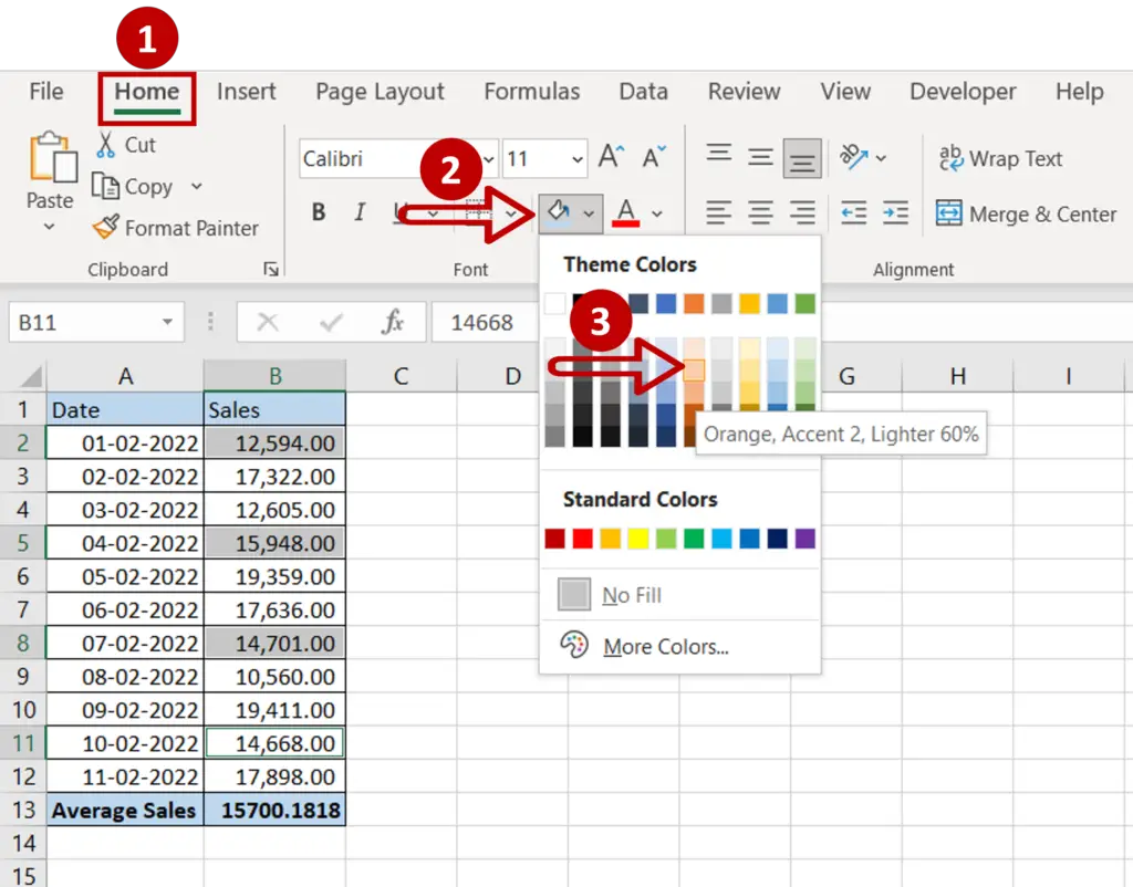
• Go to Home > Font
• Expand the Fill Color dropdown
• Select a color

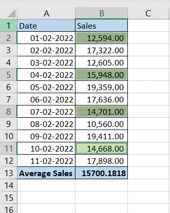
Step 3 – Check the result

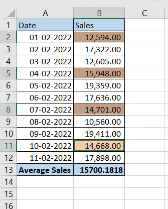
• The selected cells are highlighted

Option 2 – Use the Format Cells window

Step 1 – Select the cells

• Select the first cell to be highlighted
• Hold down the Ctrl key and click on the next cell
• Click on each of the cells to be highlighted, holding down the Ctrl key all the while

Step 2 – Open the Format Cells window

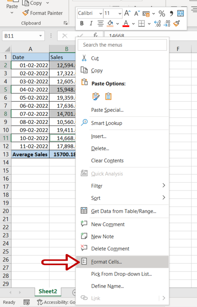
• Right-click and select Format Cells  from the context menu

OR

Go to Home > Number  and click on the arrow to expand the menu

OR

Go to Home > Cells > Format > Format Cells

OR

Press Ctrl+1

Step 3 – Choose a color

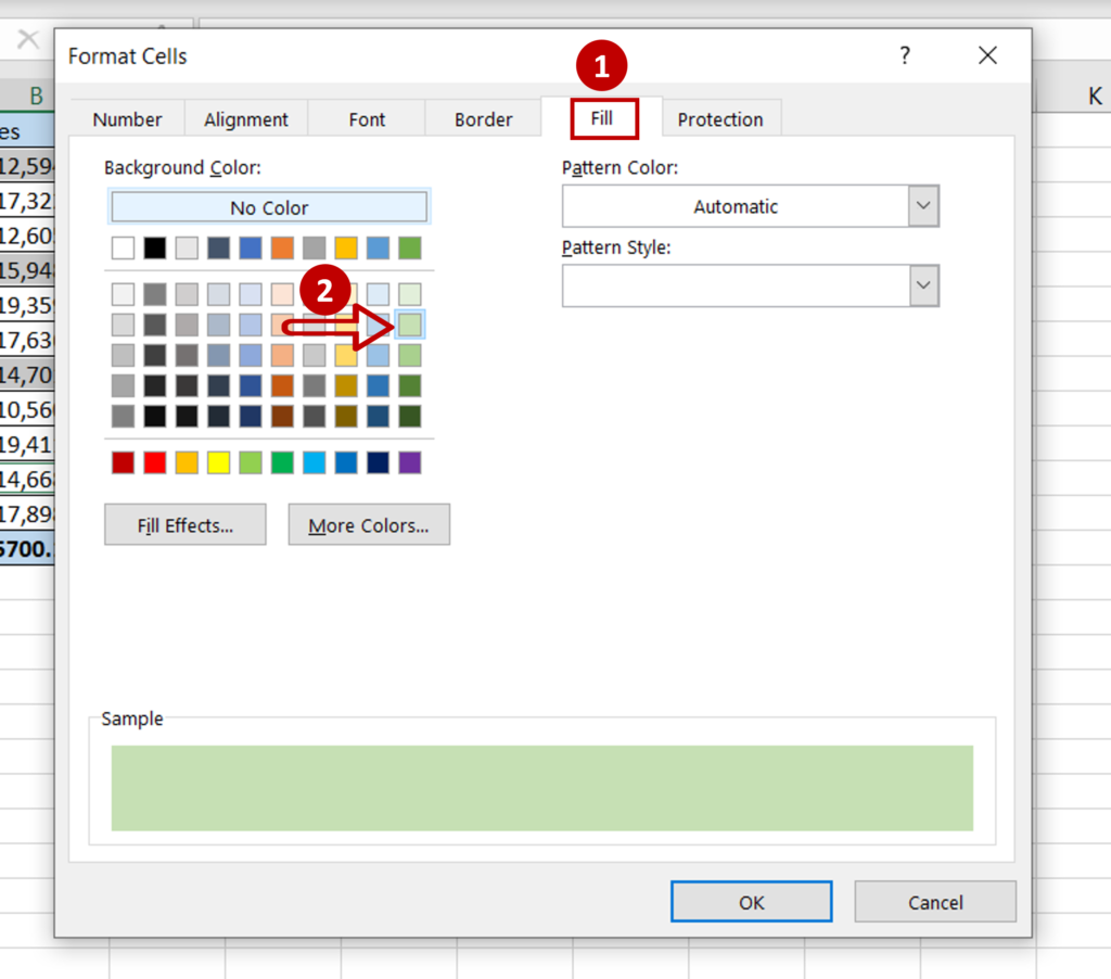
• Go to the Fill tab
• Select a color
• Click OK

Step 4 – Check the result

• The selected cells are highlighted