How to highlight numbers in Excel

You can watch a video tutorial here.

Excel has several options for formatting cells and one such option is Conditional formatting. Conditional Formatting allows you to define the format of a cell based on its value. Using conditional formatting you can set a rule to highlight numbers that meet a particular condition. Applying conditional formatting to cells is a great way to enhance a table of data by providing visual clues. You can specify a rule that can be applied to a single cell or a range of cells. The rules function based on the value in the cells and any of the following formatting can be done:

1. Highlight the cells 
2. Apply a color scale 
3. Create data bars in the cells
4. Add icons to the cells

In this example, we will look at the following options that let you change the cell color based on the value of the cells. 

1. Highlight the cells or change the color of cells that meet a condition
   1. Use a preset option
   2. Define a rule
2. Apply a color scale to all cells in a range i.e. a color gradient will be applied and the color of the cell will depend on where its value falls in relation to the other cells
   1. Use a preset option
   2. Define a rule

Option 1 – Change cell color using a preset option

Step 1 – Select the cells

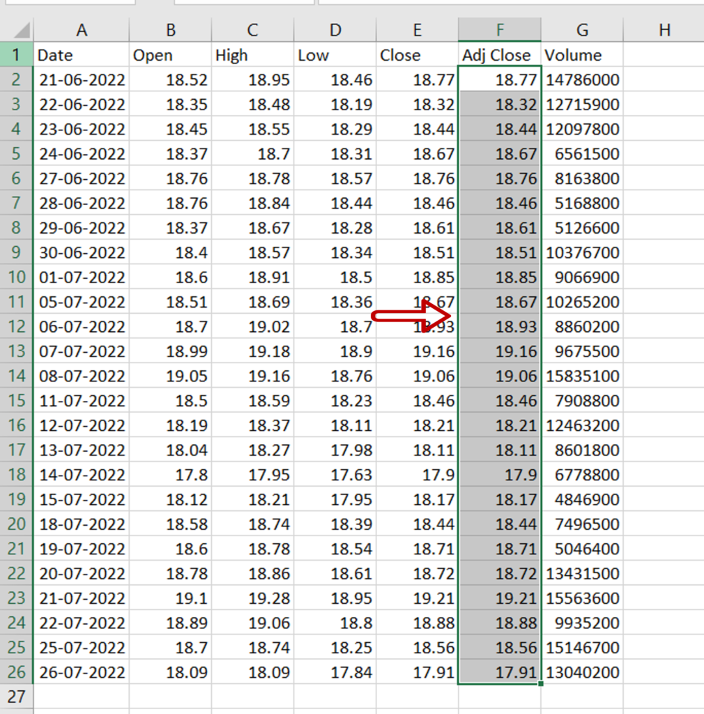
• Select the cells to be formatted

Step 2 – Choose a preset option

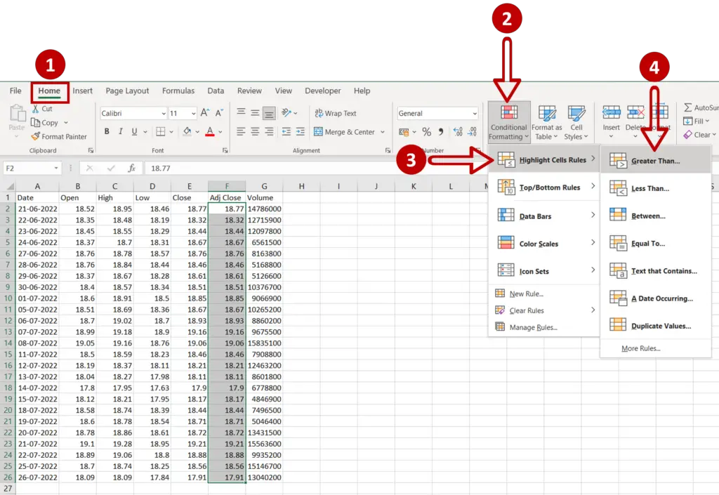
• Go to Home > Styles > Conditional Formatting
• Click on Highlight Cells Rules
• Choose Greater Than

Step 3 – Enter the value above which cells are to be highlighted

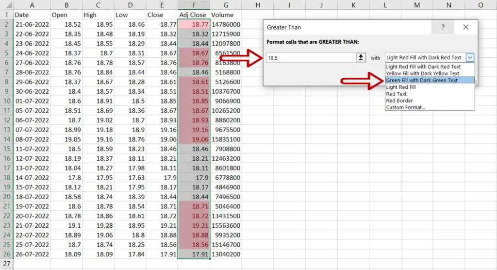
• Enter the values:

• Format cells that are GREATER THAN: 18.5 
• With: Green Fill with Dark Green Text
• Click OK

Step 4 – Check the result

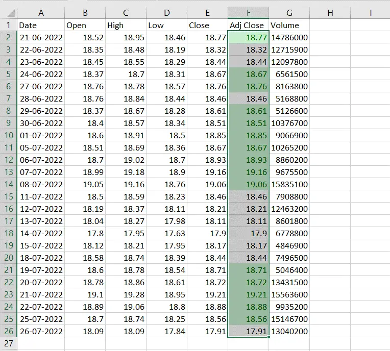
• All cells in the column that are greater than 18.5 are colored green

Option 2 – Change cell color by defining a rule

Step 1 – Select the cells

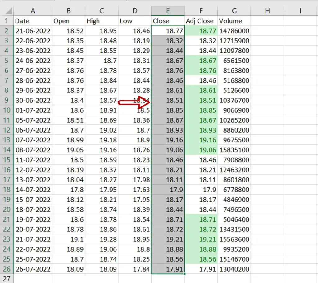
• Select the cells to be formatted 

Step 2 – Open the New Formatting Rule window

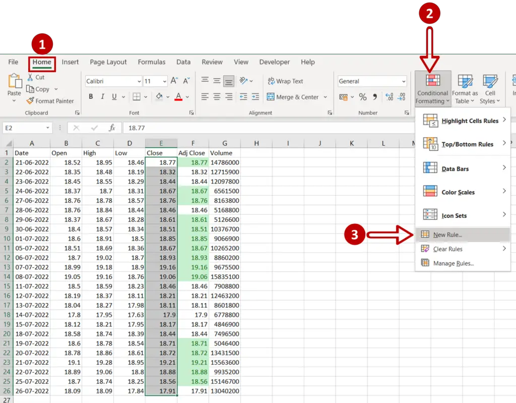
• Go to Home > Styles > Conditional Formatting
• Select New Rule

Step 3 – Set the parameters

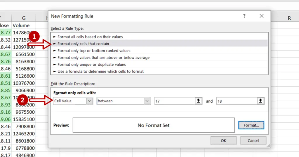
• Select Format only cells that contain
• Edit the rule description:
  • Format only cells with: Cell Value, between, 17,18
• Click Format

Step 4 – Choose the fill color

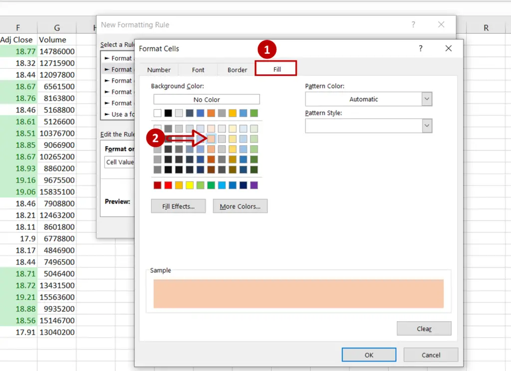
• Select the Fill tab
• Choose the color
• Click OK to close the Format Cells window
• Click OK to close the New Formatting Rule window

Step 5 – Check the result

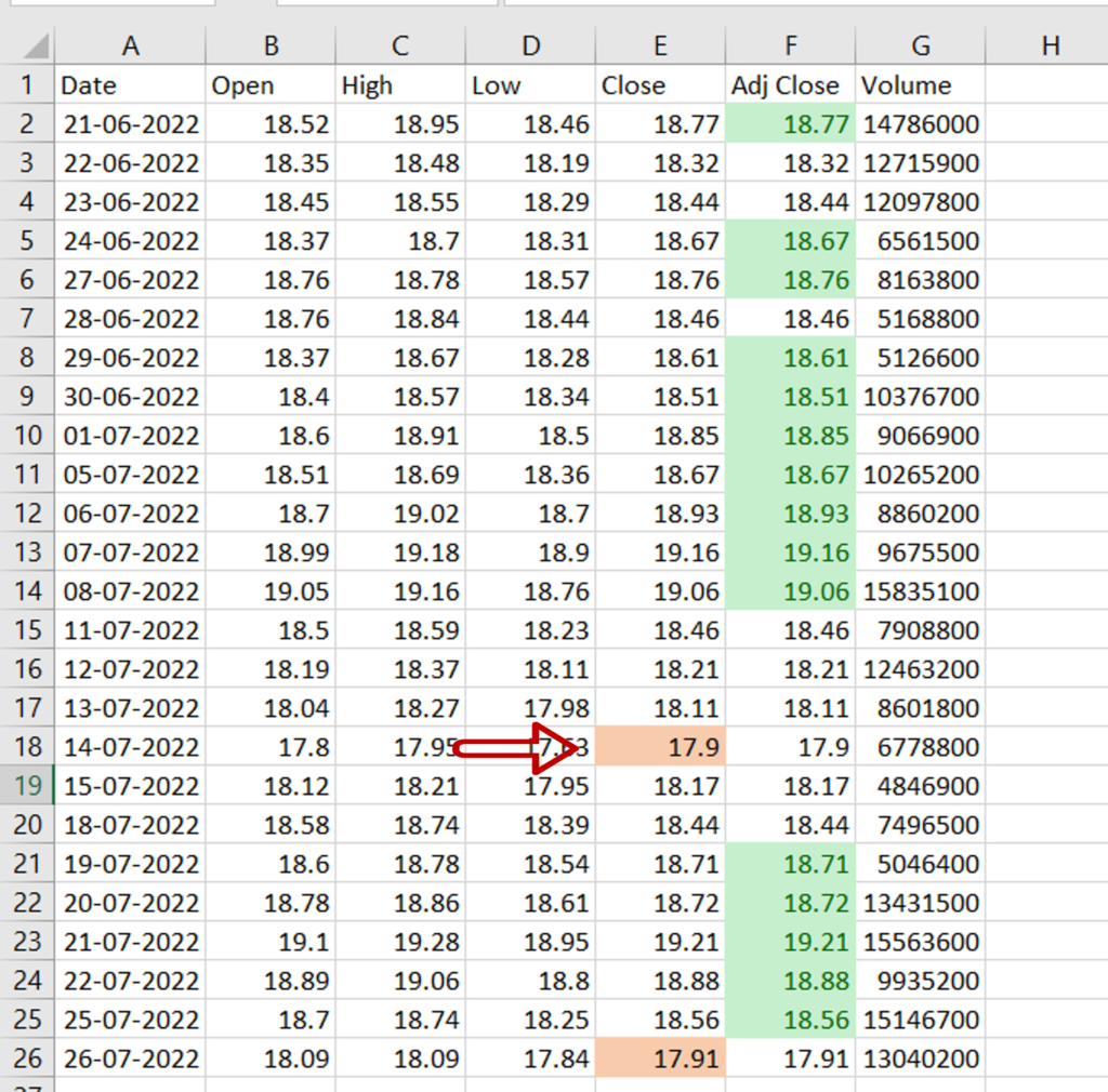
• The color has been changed of those cells whose value falls between 17 and 18

Option 3 – Apply a color scale using a preset option

Step 1 – Select the cells

• Select the cells to be formatted

Step 2 – Choose a preset option

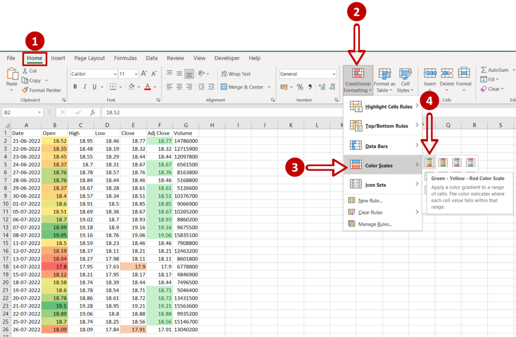
• Go to Home > Styles > Conditional Formatting
• Click on Color Scales
• Choose Green – Yellow – Red Color Scale

Step 3 – Check the result

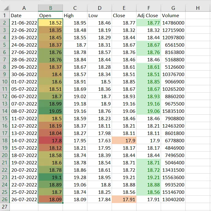
• The color gradient is applied to all the cells
• Higher values are green and lower values are red with the rest of the numbers on the color gradient in between

Option 4 – Apply a color scale by defining a rule

Step 1 – Select the cells

• Select the cells to be formatted 

Step 2 – Open the New Formatting Rule window

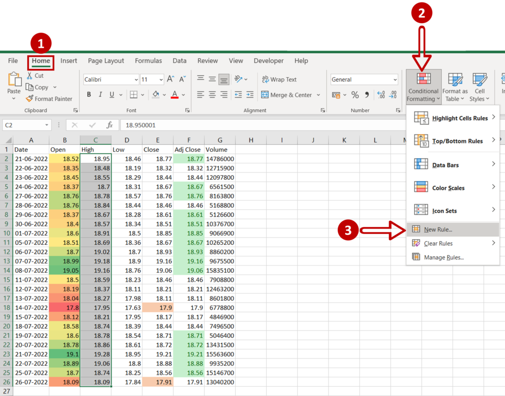
• Go to Home > Styles > Conditional Formatting
• Select New Rule

Step 3 – Set the parameters

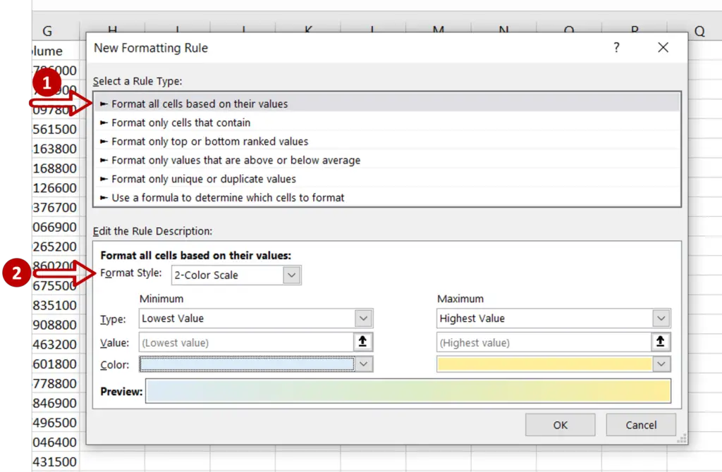
• Select Format all cells based on their values
• Under Edit the rule description:
  • Format style: 2-Color Scale
  • Type: Minimum = Lowest Value, Maximum = Highest Value
  • Select the colors scale and choose the colors
• Click OK

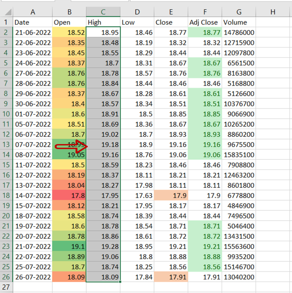
Step 4 – Check the result

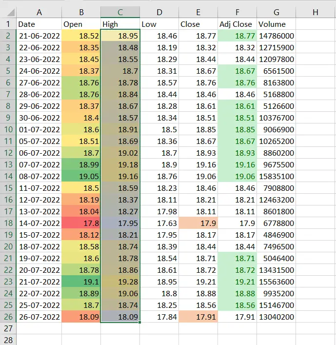
• The color gradient is applied to all the cells
• Higher values are yellow and lower values are blue with the rest of the numbers on the color gradient in between