How to highlight empty cells in Excel
You can watch a video tutorial here.

When you have a large dataset in which there are empty cells, it is not immediately apparent as to which cells are empty. Applying conditional formatting to highlight empty cells provides you with visual clues as to which cells are empty. Conditional formatting is a very useful tool that Excel provides to format cells based on their value. A rule can be set to be evaluated for a cell and the formatting of the cell changed accordingly.
Step 1 – Select the data
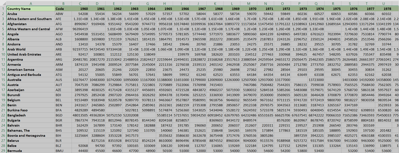
– Select the data that contains the empty cells
Step 2 – Open the New Formatting Rule box
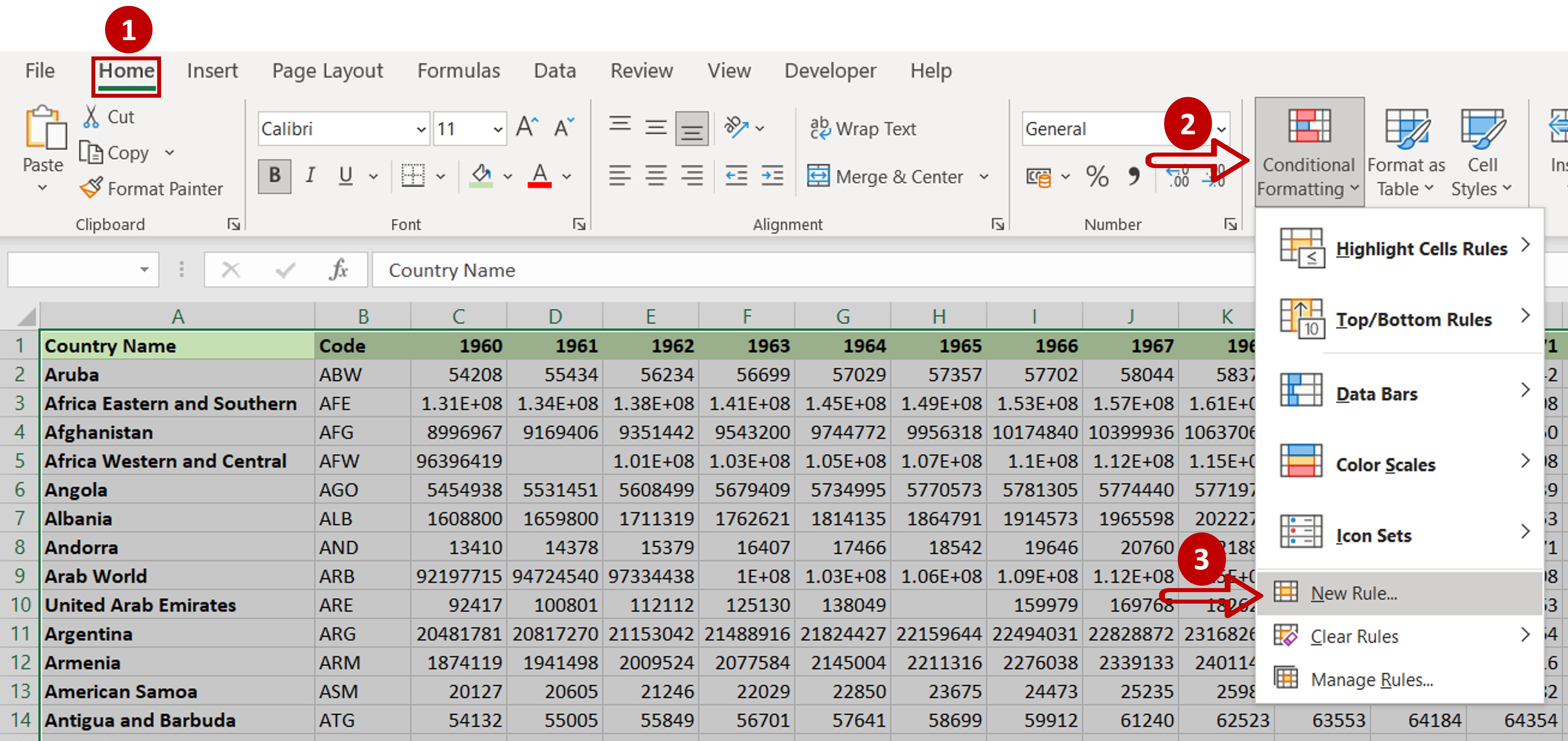
– Go to Home > Styles
– Expand the Conditional Formatting dropdown
– Select New Rule
Step 3 – Set the parameters
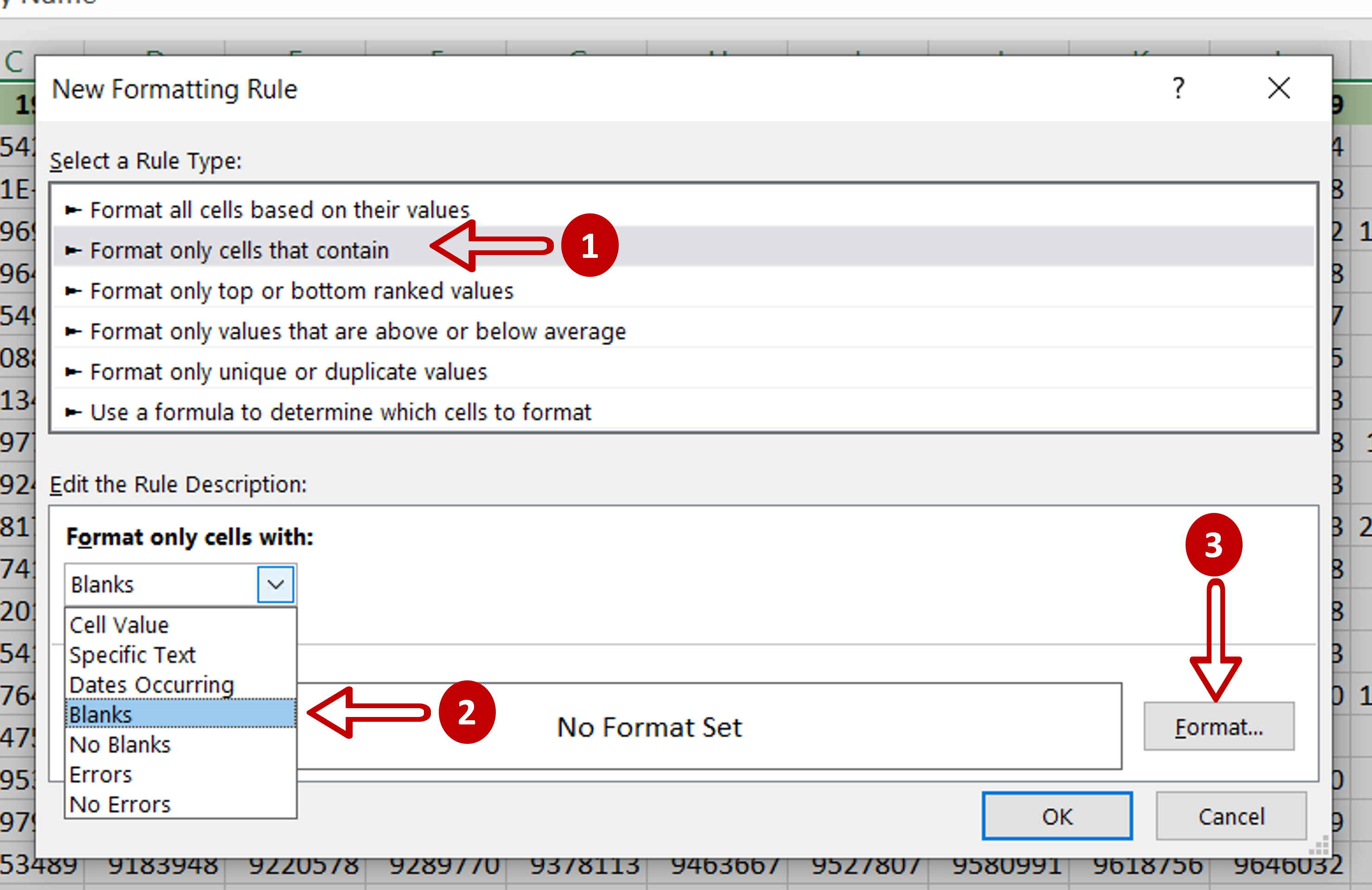
– Select Format only cells that contain
– Set ‘Blanks’ as the value for Format only cells with:
– Click Format
Step 4 – Choose the color
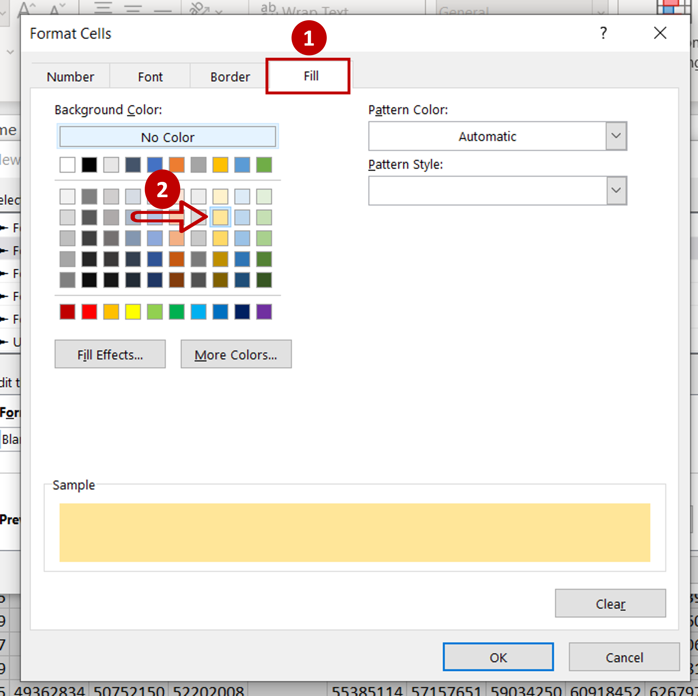
– Go to the Fill tab
– Select a color
– Click OK
– Click OK again to close the New Formatting Rule box
Step 5 – Check the result
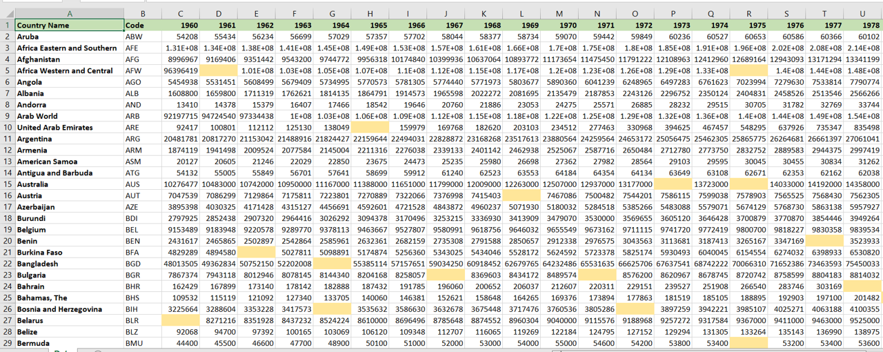
– Empty cells are highlighted with the selected color


