
How to highlight duplicate rows in Excel
 By
SpreadCheaters
By
SpreadCheaters
You can watch a video tutorial here.
When consolidating data from multiple sources, you will frequently need to check for duplicate rows. When you have a unique identifier for each record, then you can use the identifier or key to find duplicates. If you do not have a unique identifier, you will need to compare all the fields in the row to identify the duplicate records. In Excel, you can use the COUNTIFS() function with conditional formatting.
1. COUNTIFS() function: this counts the number of times the criteria is met in multiple ranges of cells
a. Syntax: COUNTIFS(range1, criteria1, range2, criteria2…….)
i. range1: the first range to be evaluated
ii. criteria1: the criteria for the first range
iii. range2, criteria2…….(optional): multiple range-criteria pairs
Step 1 – Open the New Formatting Rule box
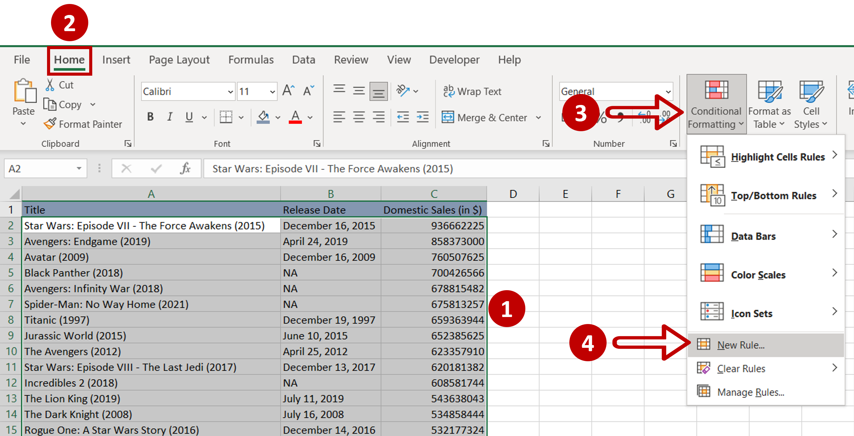
– Select the rows to be compared
– Go to Home > Styles
– Expand the Conditional Formatting dropdown
– Select New Rule
Step 2 – Create the rule
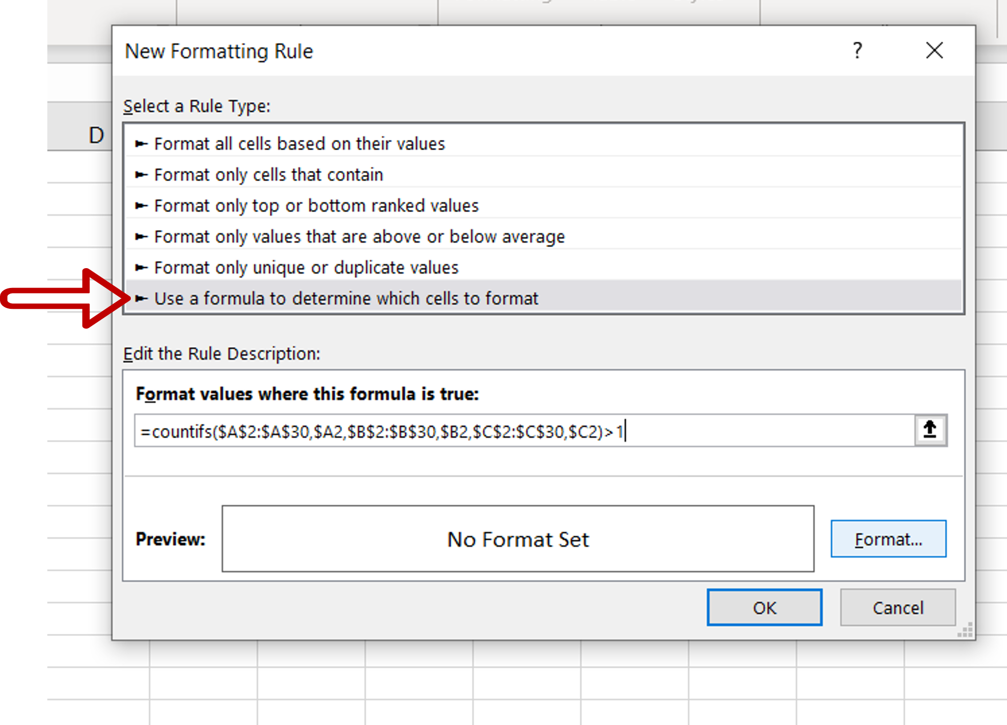
– Select Use a formula to determine which cells to format
– Under Format values where this formula is true: type the formula:
=COUNTIFS($A$2:$A$30,$A2,$B$2:$B$30,$B2,$C$2:$C$30,$C2)>1
– Click Format
Step 3 – Choose a format
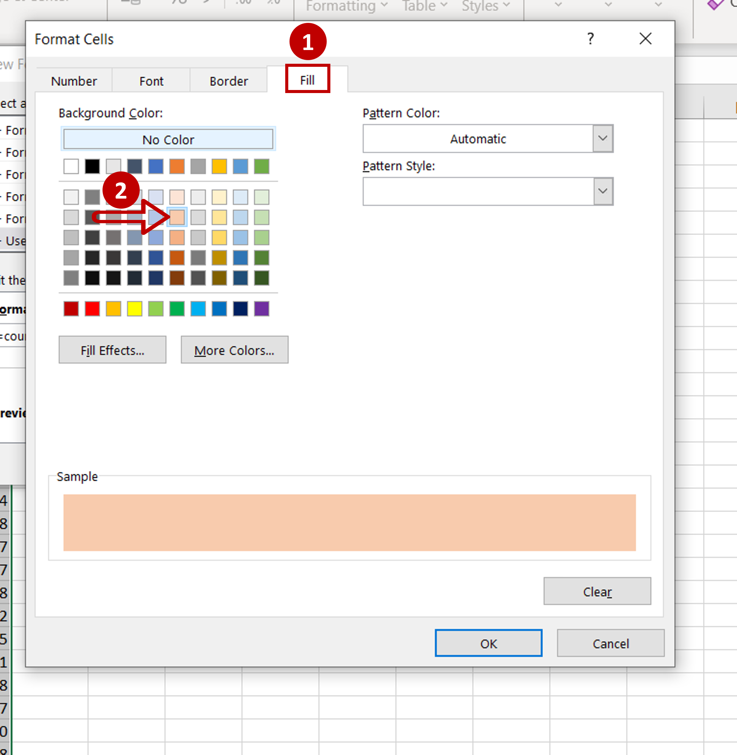
– Go to the Fill tab
– Choose a color
– Click OK
– Click OK again to close the New Formatting Rule box
Step 4 – Check the result
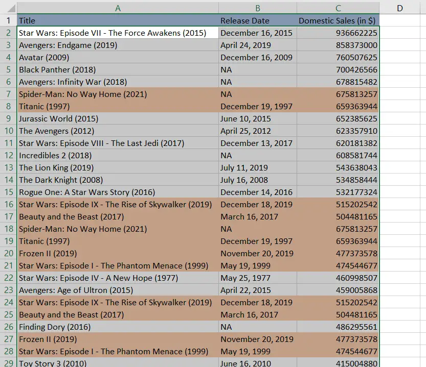
– Duplicate rows are highlighted


