How to highlight cells in Excel based on text

Highlighting cells in Excel based on text means applying a formatting rule to a group of cells to visually distinguish those cells that contain specific text from others. Highlighting cells in Excel based on text is an important feature that can improve data analysis, enhance visual clarity, save time, and provide customization options.

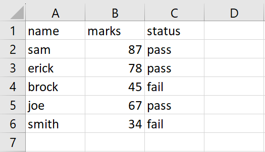
In this tutorial, we will learn how to highlight cells in Excel based on text. In our dataset, the names of students are shown along with their marks and status. We want to highlight the failed students. For this, we will use Conditional Formation. The following steps will guide you to use it.

Method 1: Highlight cells using Equal to option

Step 1 – Select the Range of cell

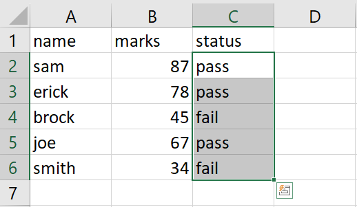
• Select the range of cells containing the cells to be highlighted

Step 2 – Click on the Conditional Formatting option

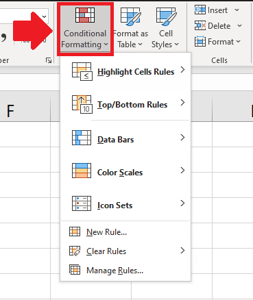
• After selecting the range of cells, click on the Conditional Formatting option and a dropdown menu will appear

Step 3 – Click on the Highlight Cell Rules option

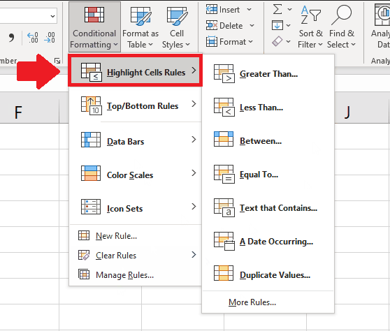
• In the dropdown menu, click on the Highlight Cell Rules option and a side menu will appear

Step 4 – Click on the Equal To option

• In the right side menu, click on the Equal To option and a dialog box will appear

Step  5 – Type the Data

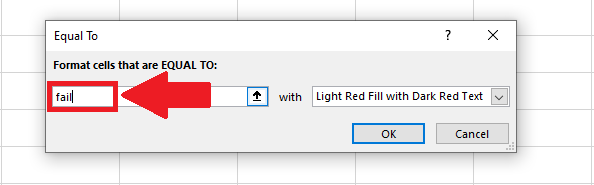
• In the dialog  box type the data to be highlighted in the box below the Format Cell that is Equal To option

Step 6 – Select the Color

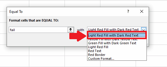
• After typing the data, select the color with which you want to highlight cells in the box next to With option 
• To select a color click on the  down arrow in the box and a dropdown menu will appear, select a color from this menu

Step 7 – Click on Ok

• After selecting the color, click on the Ok option at the end of the dialog box to get the required result 

Method 2: Highlight cells using the New Rules option

Step 1 – Select the Range of cell

• Select the range of cells containing the cells to be highlighted

Step 2 – Click on the Conditional Formatting option

• After selecting the range of cells, click on the Conditional Formatting option and a dropdown menu will appear

Step 3 – Click on the New Rule option

• From the dropdown menu, click on the New Rule option and a dialog box will appear

Step 4 – Select the type of Rule

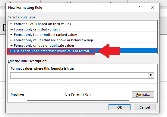
• Click on the “Use a formula to determine which cells to format” option in the list of rules in the dialog box

Step 5 – Type the formula

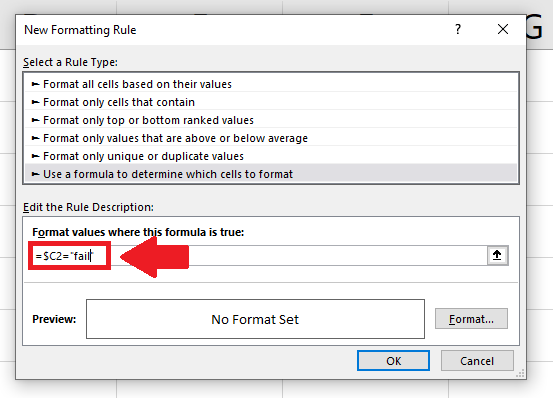
• Type “ =$C2= “fail” ” in the box below the Format values where this formula is true

Step 6 – Click on the Format option

• Click on the format option and a format cell dialog box will appear

Step 7 – Select the Color

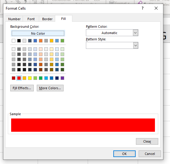
• From the dialog box, click on the color that you want to apply to the cells
• Here we have used a red color, you may use any other color
• Click on OK after selecting the color

Step 8 – Click on OK

• After selecting the color from the Format cells dialog box, Click on OK from the New Formatting Rules dialog box to get the required result