How to highlight blank cells in Excel
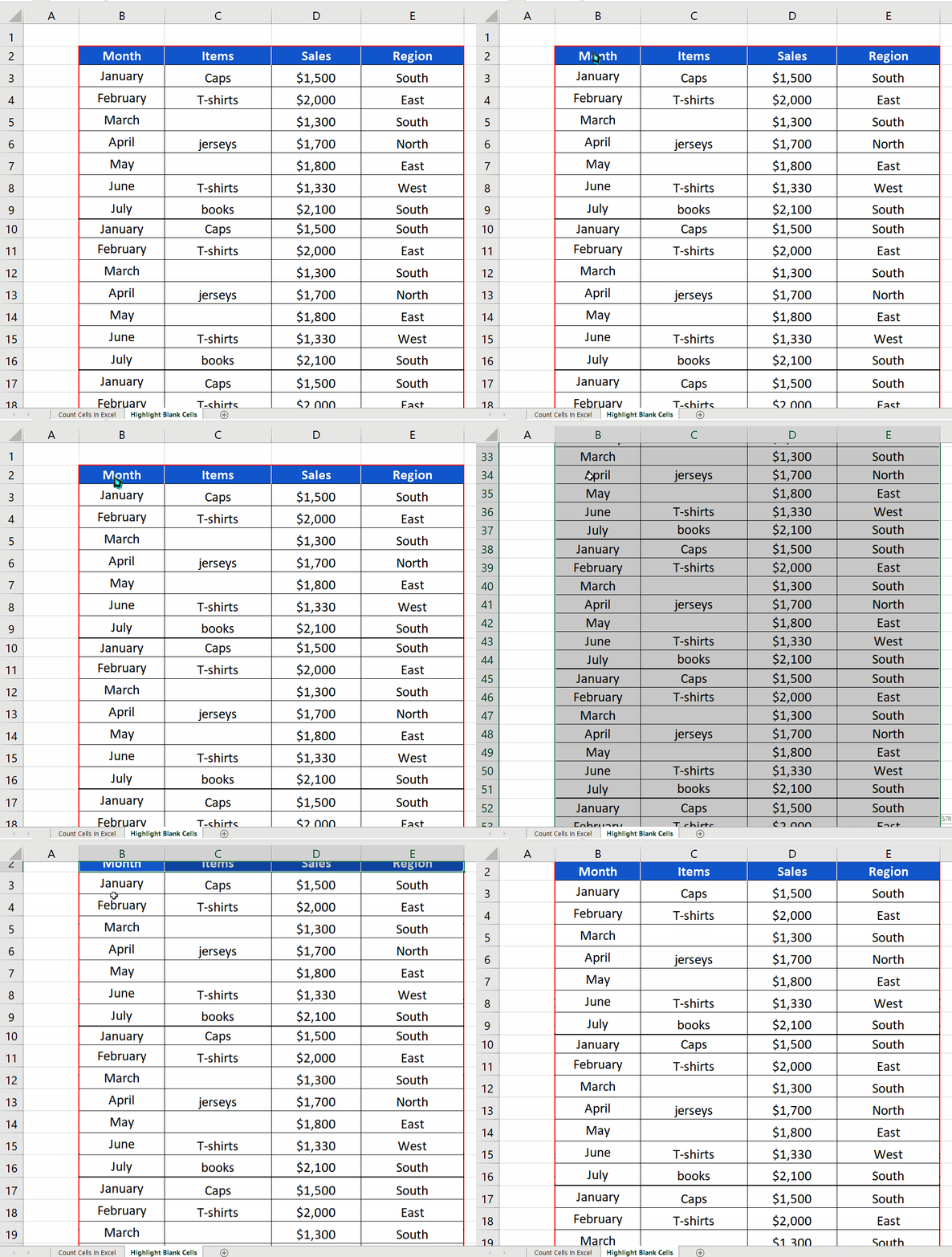
Sometimes when you are working with big datasets, you need to highlight the cells that are blanks. Excel provides us with a built-in function to check whether the cell is blank or otherwise through ISBLANK function. However, this tool has to be used with conditional formatting to highlight the blank cells in your dataset. So, in today’s tutorial we are going to learn how to highlight the blank cells in our data using ISBLANK along with conditional formatting
In the data set shown above we can see that we have 58 rows of data and there are blanks in the data as well. Imagine if this sort of data expands to 1000s of rows, then visually finding the blanks can be almost impossible. So, let’s use Excel effectively to highlight the blanks by following the steps mentioned below.
Syntax of ISBLANK
The basic syntax of ISBLANK function is as follows;
ISBLANK(value)
value: It represents the cell which is to be checked for being blank. If the cell is blank a TRUE will be returned and a FALSE will be returned in the other case.

Excel is a very powerful software when it comes to performing data analysis, mathematical, statistical or financial calculations. It also has a wide variety of functions and tools that help us to visualize the data for better analysis. Especially, if we are working with large datasets then better visualization and representation makes it easier to analyze the data.
Step 1 – Select the complete data range

– We’ll have to select the whole data range first because we will apply the conditional formatting on all of it. If the data range is small, selection can be done manually. However, if the data range is very large then select the first cell just beneath the header row and press CTRL+SHIFT+ right arrow button to select all columns and then CTRL+SHIFT+ down arrow button to select all the rows as shown above.
Step 2 – Locate the New Rule option in conditional formatting
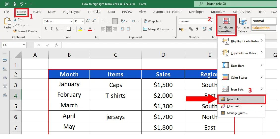
– On the HOME tab, go to the Styles group and click on the Conditional Formatting dropdown arrow.
– Select New Rule option as shown above.
Step 3 – Choose Use a formula and write the formula
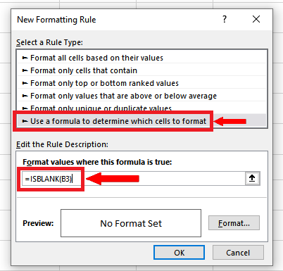
– In the New Formatting Rule dialog box select the last option Use a formula to determine which cells to format.
– Enter the following formula in the Format values where this formula is true,
=ISBLANK(B3)
This tells excel to check every cell in the selected range to be a blank. Whenever a blank cell is found this formula will produce a TRUE result.
Step 4 – Set the format for highlighting blank cells
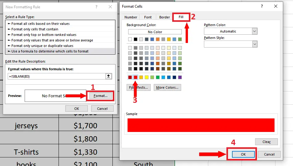
– In the New Formatting Rule dialog box after writing the formula, click on the Format button.
– This will open up a new dialog box, choose an appropriate fill color to highlight the blank cells and press the OK button.
Step 5 – Implement the conditional formatting to highlight blank cells
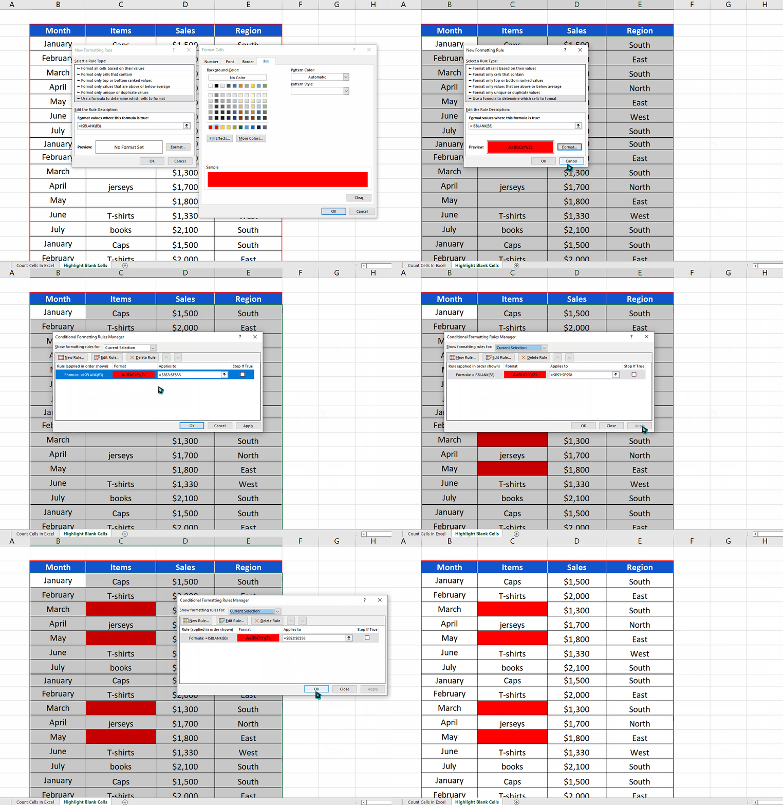
– After choosing the appropriate color and in Format Cells press OK button and then again press OK button on New Formatting Rule.
– It will lead you to another dialog box click on the Apply button to see the effect of conditional formatting and then finally press the OK button to implement the conditional formatting as shown above.


