
How to hide rows in Excel based on cell value
 By
SpreadCheaters
By
SpreadCheaters
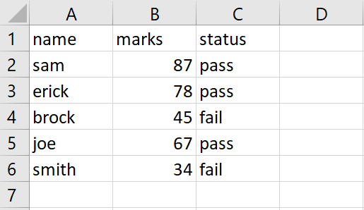
In this tutorial, we will learn how to hide rows in excel based on cell value. In our dataset, we have the results of students. We want to show only the passed students and hide the failed students. For this, we will use the Sort and Filter option. The following steps will guide you to use this option.
Hiding rows in Excel based on a cell value means making certain rows in a worksheet invisible, based on the value in a particular cell or range of cells. Hiding rows in Excel based on cell values is a useful feature that can help you manage and organize your data more effectively, while also improving the security and clarity of your spreadsheets.
Step 1 – select the range of cells
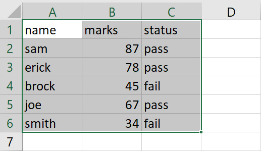
– Select the range of data that contains the rows that you want to hide
Step 2 – Click on the Sort and Filter option
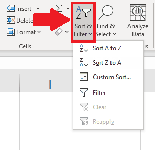
– After selecting the range of cells, click on the Sort and Filter option in the Editing group of the Home tab, and a drop-down menu will appear
Step 3 – Click on the Filter option
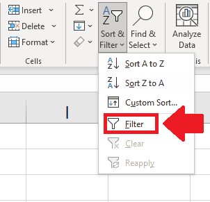
– In the drop-down menu, click on the Filter option
Step 4 – Click on the Down Arrow
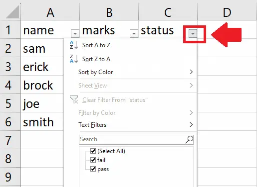
– Click on the Down Arrow in the first cell of the selected range and a dialog box will appear
Step 5 – Uncheck the un necessary Data
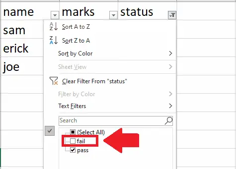
– In the dialog box, uncheck the data that you want to hide
Step 6 – Click on OK

– Click on OK at the end of the dialog box to get the required result


