
How to get y=mx+b on Excel
 By
SpreadCheaters
By
SpreadCheaters
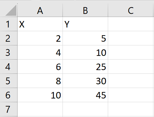
In our dataset, we have two sets of numerical values: X and Y. Our goal is to establish a linear equation of the form y=mx+c that best fits the relationship between X and Y. To achieve this, we will create a chart of the X and Y data points, and then apply a trend line to the chart that best fits the data. Finally, we will display the equation of the trend line on the chart.

“y=mx+b” is a mathematical formula for a linear equation, where “y” represents the dependent variable, “x” represents the independent variable, “m” represents the slope of the line, and “b” represents the y-intercept. In Excel, Finding the equation of a line in the form of “y=mx+b” is a fundamental tool in data analysis, modeling, and prediction, and has numerous applications in various fields.
Step 1 – Select the range of cell
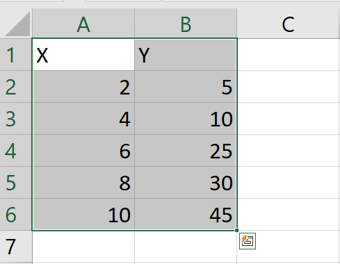
– Select the data by using the “Handle select” and “Drag and Drop” method
Step 2 – Apply a Scatter Chart
– After selecting the range of cells, Click on the Scatter Chart option in the Charts group of the Insert tab, and a chart will appear on the sheet
Step 3 – Click on Chart Elements
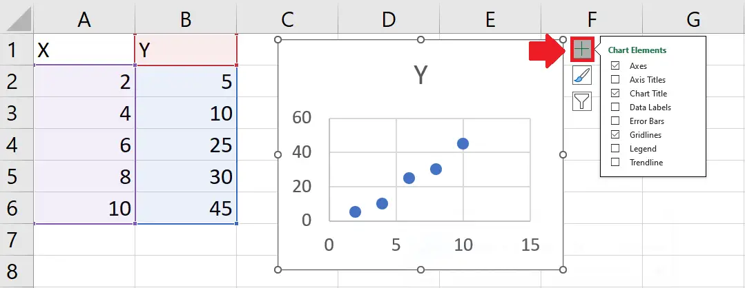
– Click on the chart
– After clicking on the chart Chart Elements will appear at top of the chart
– Click on chart Element and a right-side menu will appear
Step 4 – Click on the Trend Line option

– In the right side menu, click on the TrendLine option to add a trend line to the chart
Step 5 – Click on More Options
– Click on the arrow next to the Trendline option and a right-side menu will appear
– From this menu, click on More Options, and a Format Trendline dialog box will appear on the right side of the sheet
Step 6 – Click on the Display equation option
– In the right-side menu click on the Display the Equation on the Chart option to get the required result
– In our case m:5 and b:-7


