
How to get rid of div 0 in Excel
 By
SpreadCheaters
By
SpreadCheaters
You can watch a video tutorial here.
Excel has a setting that checks for errors when data is entered into a worksheet. A small green triangle appears in the upper left corner of the cell and when the cell is selected a warning icon is displayed. The DIV 0 error is displayed when you try to divide a number by zero. This error alerts you to a possible mistake in the formula so that you can correct it. More often than not, the formula is correct but the error is displayed. In this example, we will see how to get rid of the error using the IFERROR() function.
When you create a formula in which you know that some calculations will result in the DIV 0 error, it is better to encase it in the IFERROR() function.
1. IFERROR(): this returns a specified value if the formula or condition results in an error.
a. Syntax: IFERROR(condition, value)
i. condition: the condition to be evaluated
ii. value: the value to be returned if the condition returns an error
Step 1 – Edit the formula
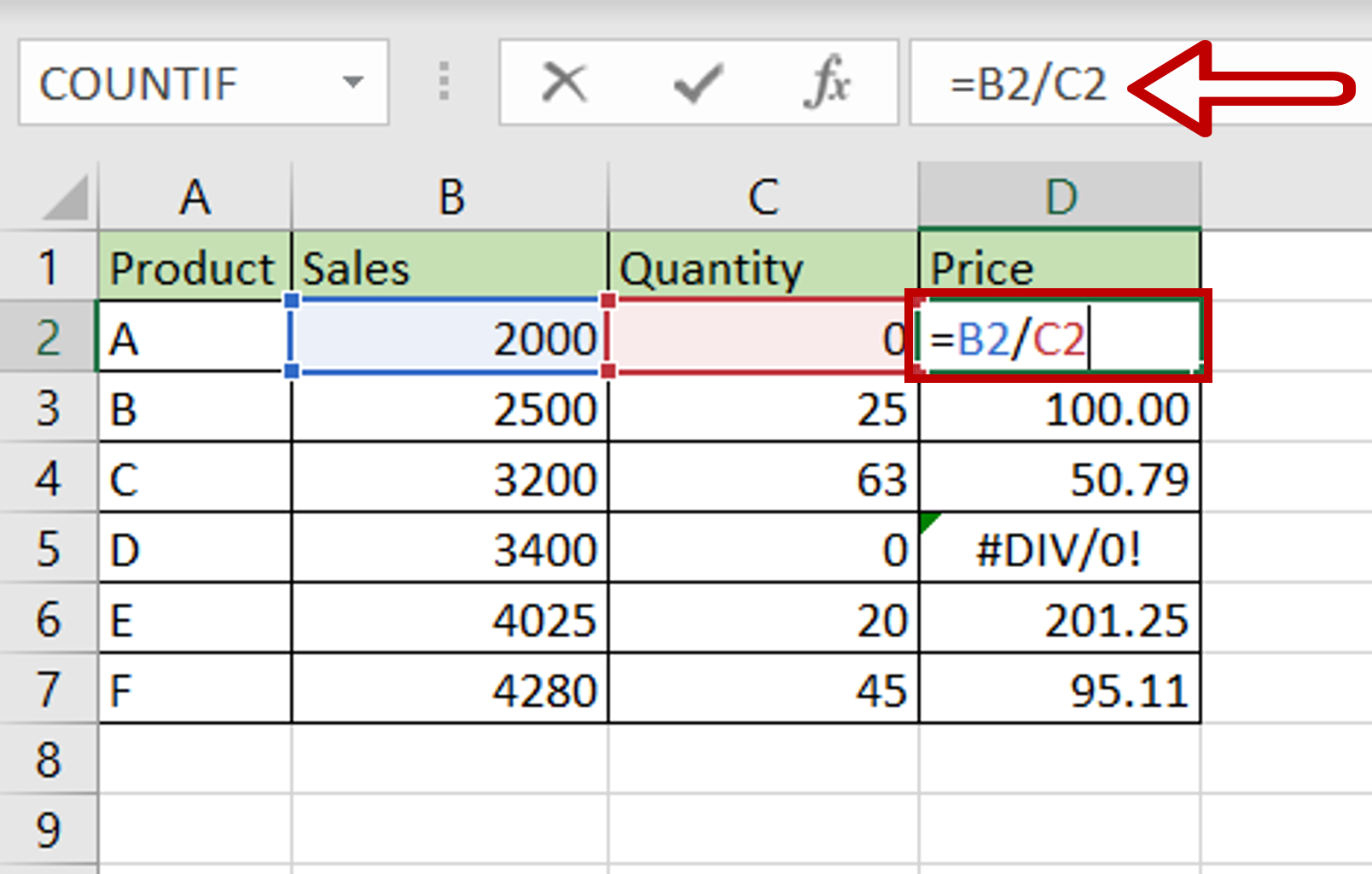
– Select the first cell with the formula that is showing an error
– Press F2 to enable the cell for editing or place the cursor in the formula bar
Step 2 – Add the IFERROR() function
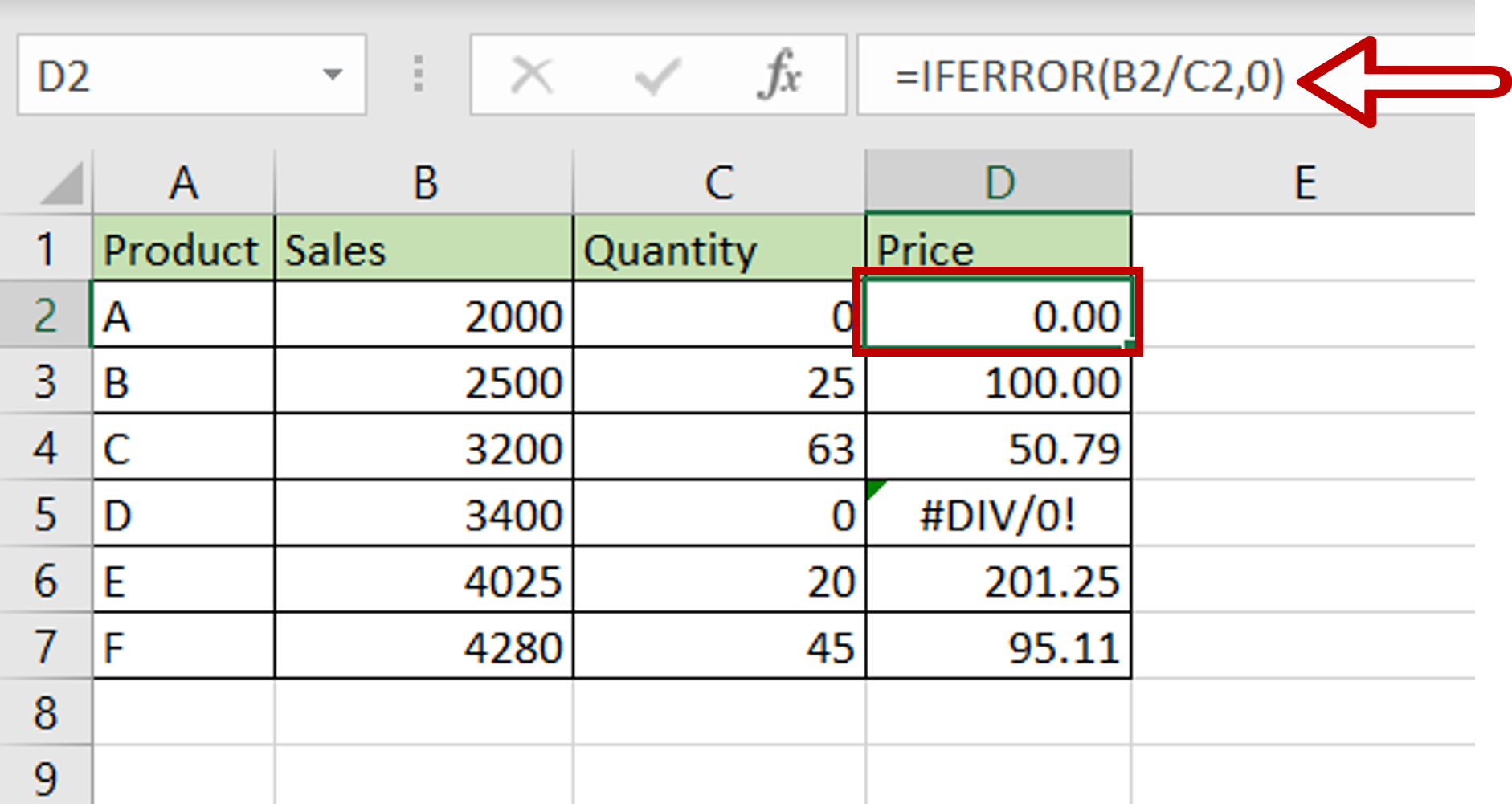
– Enhance the formula as follows:
=IFERROR(Sales/Quantity,0)
– The value is given as zero so that a zero is returned in case the formula results in the DIV 0 error
– Press Enter
Step 3 – Copy the formula
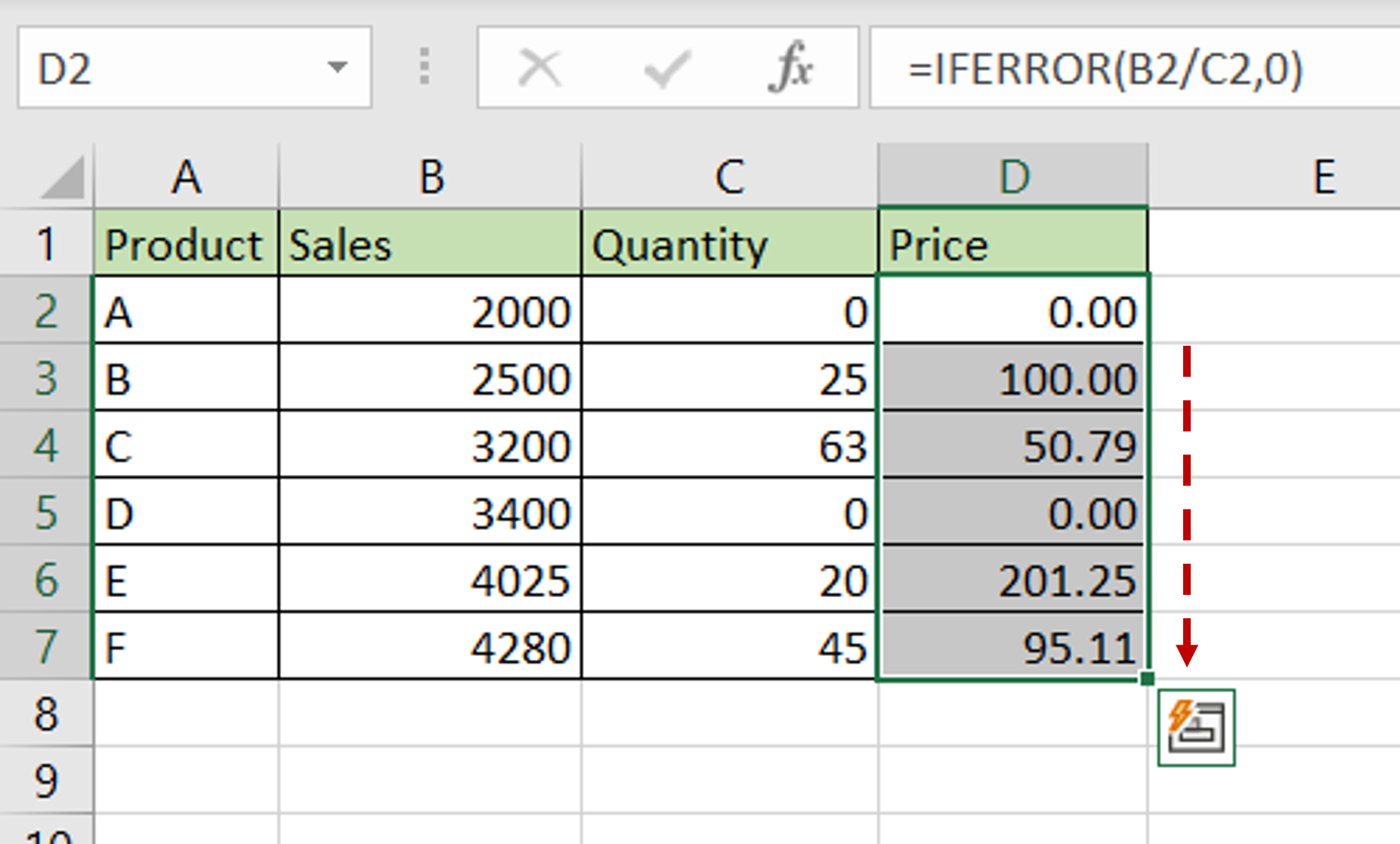
– Using the fill handle from the first cell, drag the formula to the remaining cells
OR
a) Select the cell with the formula and press Ctrl+C or choose Copy from the context menu (right-click)
b) Select the rest of the cells in the column and press Ctrl+V or choose Paste from the context menu (right-click)
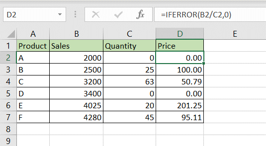
Step 4 – Check the result

– Wherever the formula requires the number to be divided by zero, zero is displayed instead of the DIV 0 error message


