
How to generate random name pairs in Excel
 By
SpreadCheaters
By
SpreadCheaters
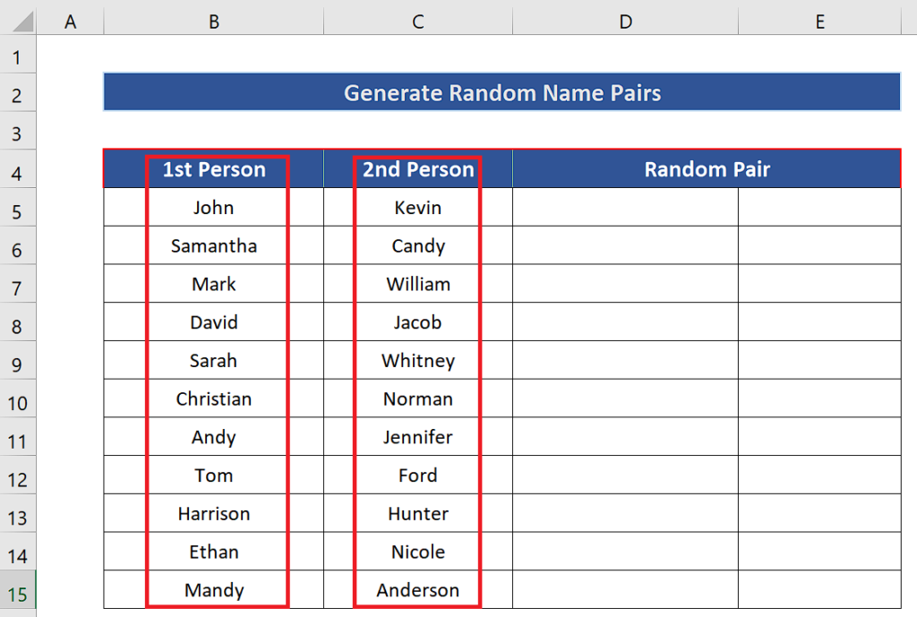
Here is the dataset and it contains two lists of names and we’ll learn to create a method using Excel’s built-in functions to generate a list of random name pairs.

Excel provides us with a very handy function to produce random numbers. There is a good variety of functions available to produce random numbers in Excel. However, there is no direct function available to produce random text or names, but sometimes we need to generate random pairs or names for creating new teams for a group task. In that case, you’ll have to follow the steps mentioned below to create a list of random names of people from two different lists.
Step 1 – Insert two columns in the dataset
– To insert the columns in between the list of names, select the column before which you wish to insert the column.
– Now press CTRL + SHIFT + Plus Key (+). This will insert a column to the left of the selected column.
– Repeat the above step to insert one more column as shown above.
Step 2 – Use RAND to create an array of random numbers
– Select all the cells of newly added columns, starting from the top left cell of the newly added columns only.
– Write the following formula in the top left cell while keeping all cells selected.
– Now enter the formula while pressing CTRL+SHIFT+ENTER. This will implement the formula in all the cells and an array of random numbers will be generated as shown above.
Step 3 – Use SORTBY function to create a random list
– Now we’ll use the SORTBY function which allows us to sort an array with respect to another array. We’ll sort the names of 1st persons with respect to the random numbers in the first column. Following will be the formula,
=SORTBY(B5:B15,C5:C15,1)
B5:B15 is the range representing the names of 1st persons and C5:C15 are the random numbers generated by Excel. The last 1 tells Excel to sort the names in ascending order with respect to the random numbers in C5:C15.
– Repeat the same process with second list of names and use the appropriate formula, for our case the second formula will be,
=SORTBY(E5:E15,D5:D15,1)
– We’ll get the random name pairs in columns F and G. If you want to change the pairs just press F9 and new random pairs will be generated as shown above.


