
How to freeze panes in Excel
 By
SpreadCheaters
By
SpreadCheaters
You can watch a video tutorial here.
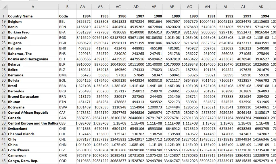
Freezing a pane is commonly used when scrolling through large amounts of data on a worksheet. When scrolling through a sheet that has a lot of data and either column headers or row names, it is difficult to keep track of the name of the row or column. Freezing either a row or column makes it possible to keep the row name or column header in place while you scroll through the rest of the data.
Step 1 – Navigate to the Freeze Panes option
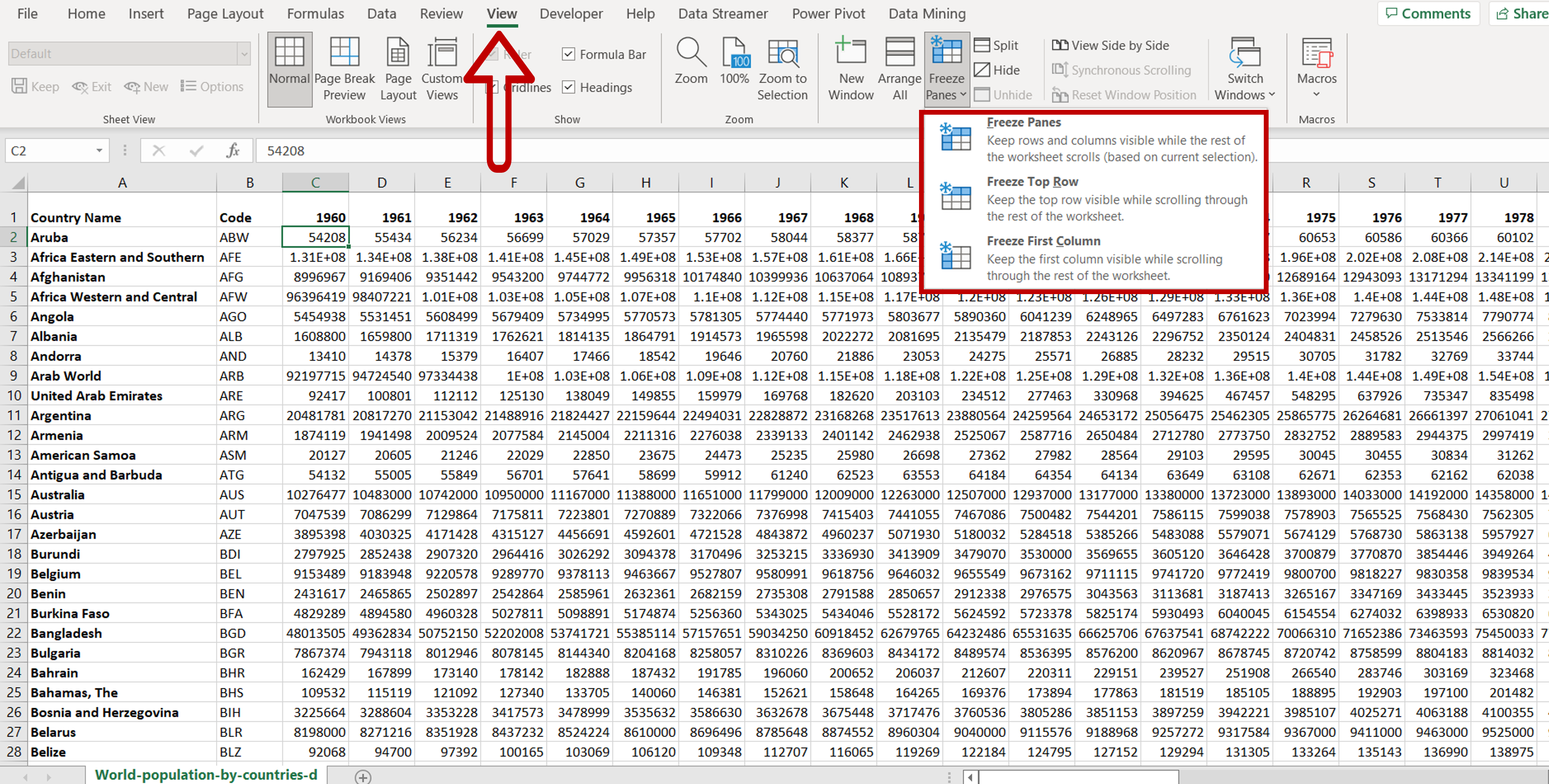
– Select the View menu
– Select the Freeze Panes option on the Window section
Step 2 – Select the appropriate option
– Position the cursor at the location of which the rows above and columns to the left are to be locked
– Select the Freeze Panes option from the menu
– The Freeze Top Row option locks Row 1 and the Freeze First Column option freezes column
A. The position of the cursor does not matter in these cases.
Step 3 – Unfreeze the Panes
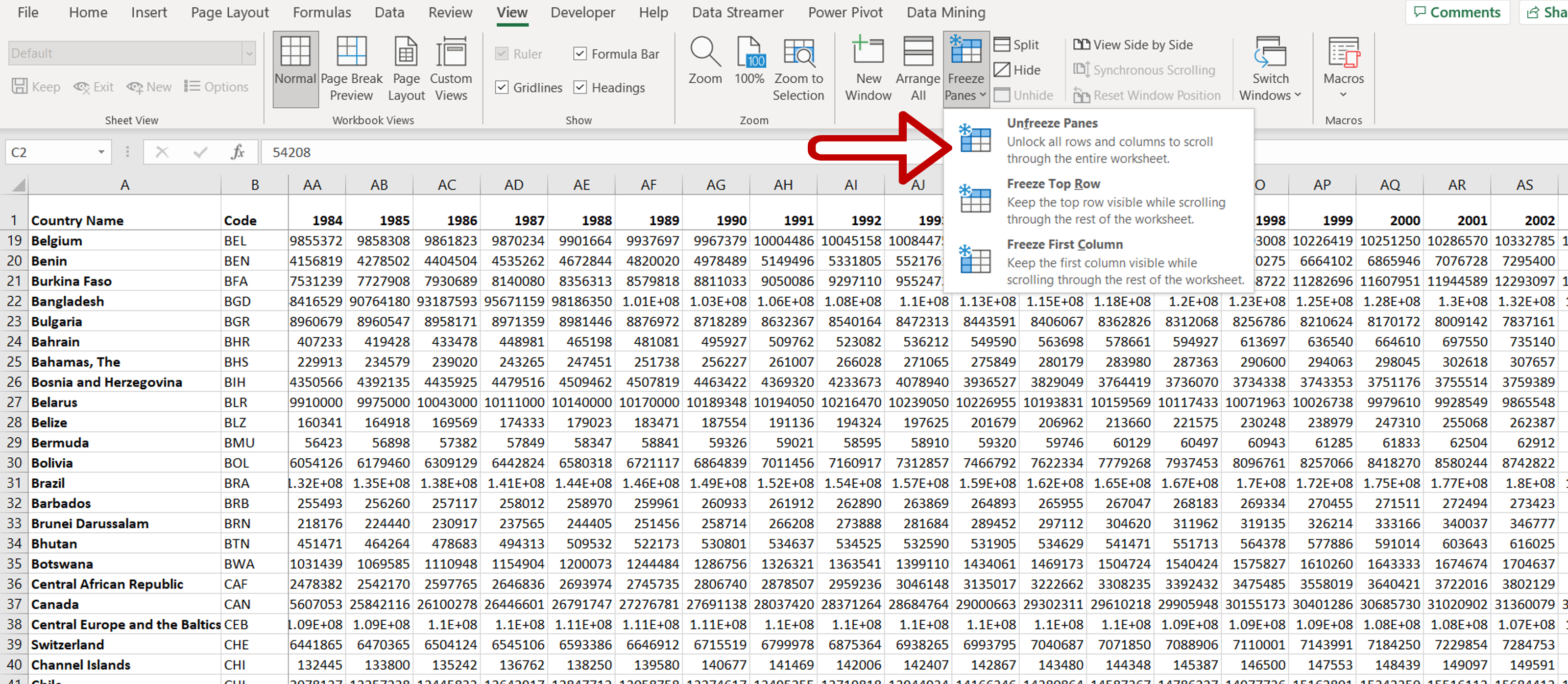
– To unlock the frozen rows/columns, navigate to the Freeze Panes menu
– Select the Unfreeze Panes option


