
How to freeze multiple panes in Excel
 By
SpreadCheaters
By
SpreadCheaters
Page last updated:
06/12/2022 |
Next review date:
06/12/2024
You can watch a video tutorial here.
Freezing a pane is commonly used when scrolling through large amounts of data on a worksheet. When scrolling through a sheet that has a lot of data and either column headers or row names, it is difficult to keep track of the name of the row or column. Freezing either a row or column makes it possible to keep the row name or column header in place while you scroll through the rest of the data.
Step 1 – Select the source
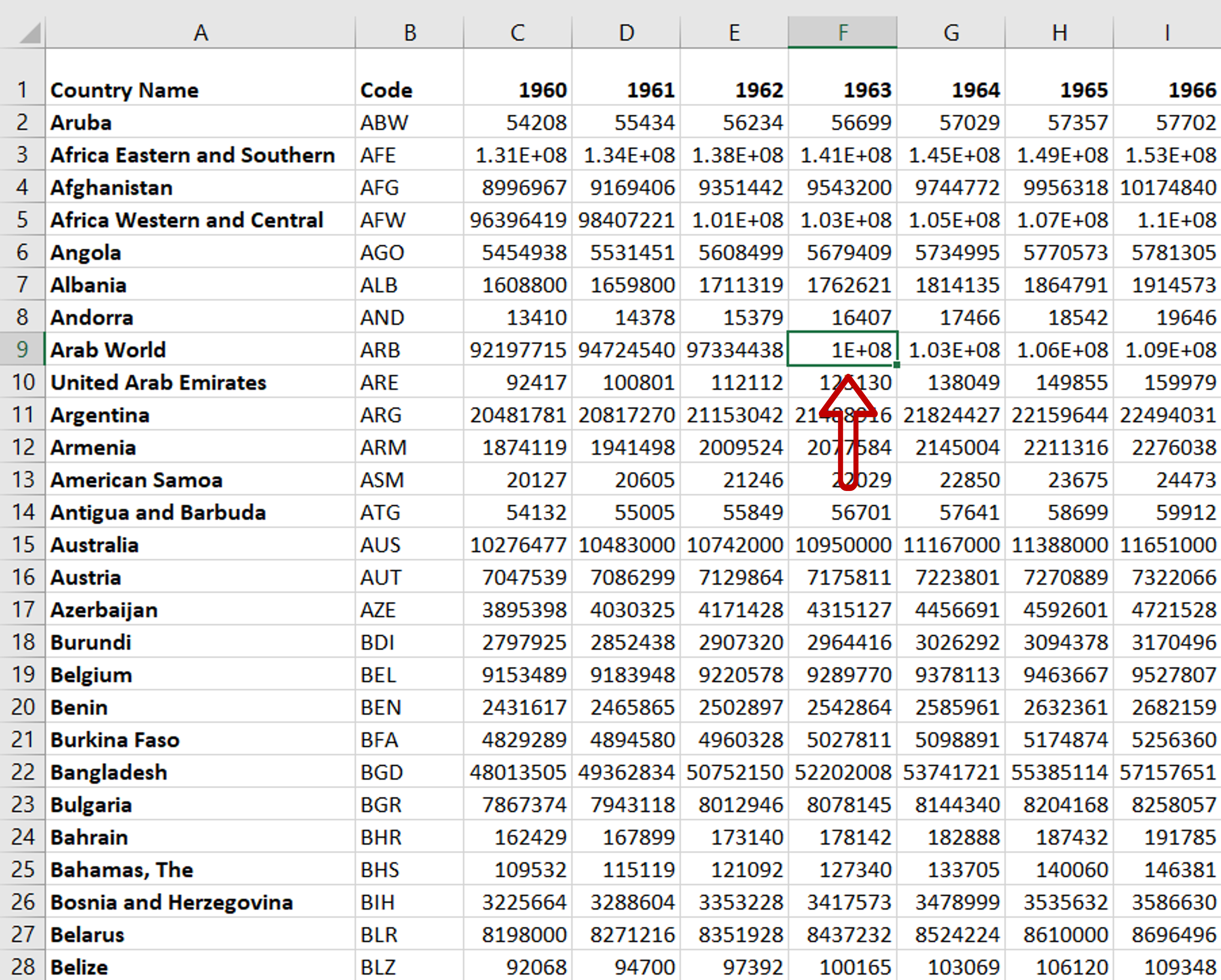
– Select the cell at the location of which the rows above and columns to the left are to be locked
Step 2 – Navigate to the Freeze Panes option
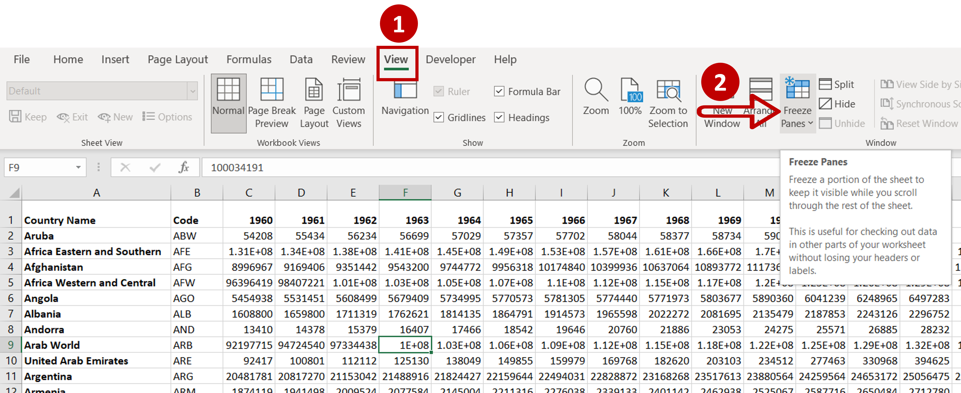
– Go to View > Window
– Expand the Freeze Panes dropdown
Step 3 – Choose an option
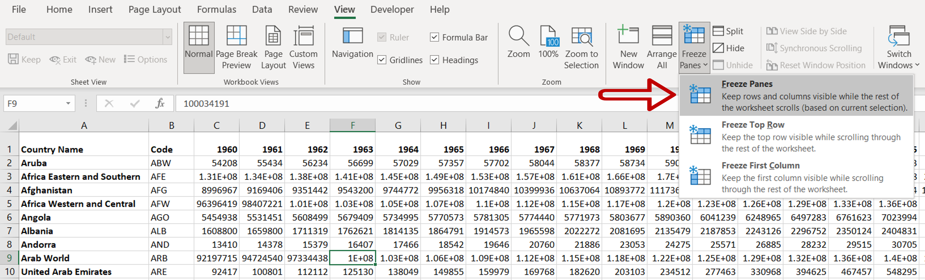
– Select Freeze Panes
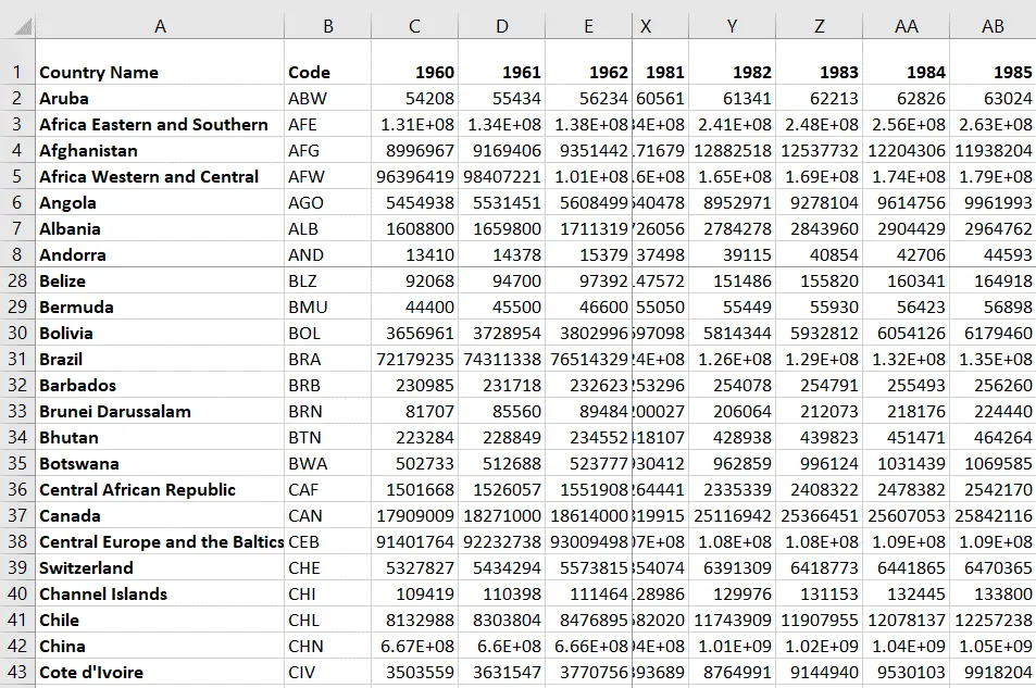
Step 4 – Check the result
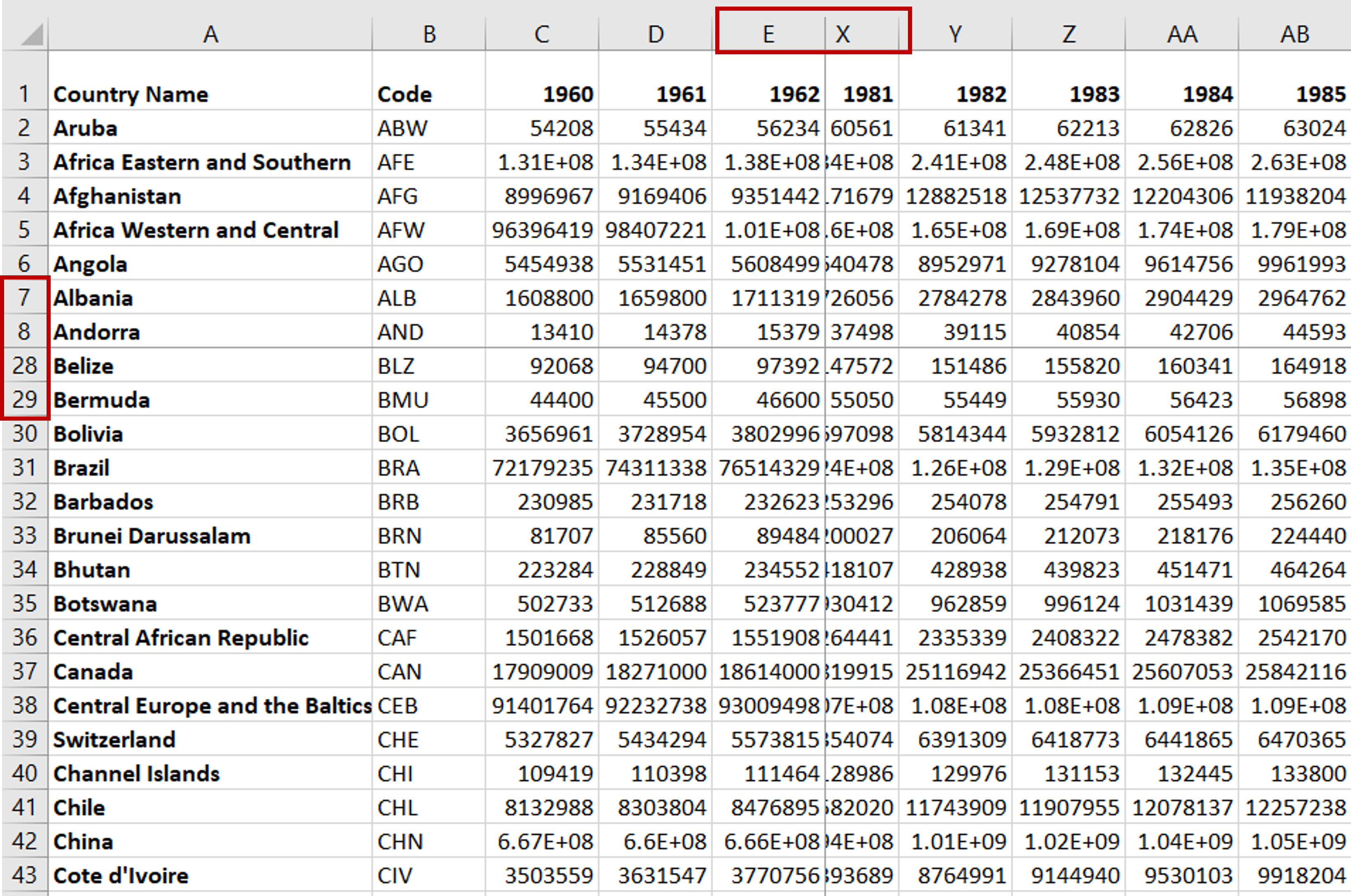
– Scroll to the right
– Scroll down
– Multiple panes above and to the left of the cursor remain frozen


