
How to freeze data up to second row in Excel
 By
SpreadCheaters
By
SpreadCheaters
Freeze data up to second row:
By making some rows static, we can scroll through the other rows of data while keeping the desired rows visible all the time.
To do this yourself, please follow the steps described below;
Microsoft Excel offers some very interesting features to handle large data sets. These features are very handy when we want to navigate through the data in an Excel workbook with a big data set, i.e. rows and columns of the order of 100s to 1000s. One of these features is freezing any number of rows we want to stay visible all the time.
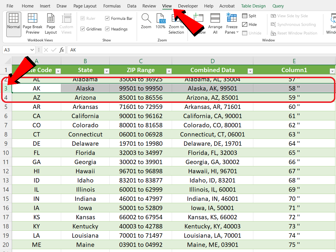
Step 1 – Select the third row to freeze data upto second row in Excel
– Open the desired workbook in which you want to freeze the data upto second row.
– As we wish to freeze the second row so we have to select the complete third row by clicking on row index ‘3’.
– Now navigate to “View Tab” from the list of tabs available at the top row as shown below;
Step 2 – Freezing the data up to second row

– In “View Tab”, locate “Freeze Panes” and choose “Freeze panes” as shown below, and you are done. The data up to second row is frozen now.


